The stochastic model describes a situation where uncertainty is present. In other words, the process is characterized by some degree of randomness. The adjective "stochastic" itself comes from the Greek word for "guess." Since uncertainty is a key characteristic of everyday life, such a model can describe anything.
However, each time we apply it, it will produce a different result. Therefore, deterministic models are used more often. Although they are not as close as possible to the real state of affairs, they always give the same result and make it easier to understand the situation, simplify it by introducing a set of mathematical equations.
The main signs
A stochastic model always includes one or more random variables. She seeks to reflect real life in all its manifestations. Unlike stochastic, it has no goal to simplify everything and reduce it to known values. Therefore, uncertainty is its key characteristic. Stochastic models are suitable for describing anything, but they all have the following characteristics in common:
- Any stochastic model reflects all aspects of the problem for the study of which it was created.
- The outcome of each of the phenomena is uncertain. Therefore, the model includes probabilities. The correctness of the general results depends on the accuracy of their calculation.
- These probabilities can be used to predict or describe the processes themselves.
Deterministic and Stochastic Models
For some, life seems to be a sequence for others - processes in which a cause determines an effect. In fact, it is characterized by uncertainty, but not always and not in everything. Therefore, it is sometimes difficult to find clear distinctions between stochastic and deterministic models. Probabilities are quite subjective.

For example, consider a coin toss situation. At first glance, there seems to be a 50% chance of getting tails. Therefore, you need to use a deterministic model. In reality, however, it turns out that a lot depends on the players' sleight of hand and the perfect balancing of the coin. This means that you need to use a stochastic model. There are always parameters that we do not know. In real life, a cause always determines an effect, but there is also some degree of uncertainty. The choice between using deterministic and stochastic models depends on whether we are willing to give up - simplicity of analysis or realism.
In chaos theory
Recently, the concept of which model is called stochastic has become even more blurred. This is due to the development of the so-called chaos theory. It describes deterministic models that can give different results with a slight change in the initial parameters. This is like an introduction to uncertainty calculation. Many scientists have even assumed that this is already a stochastic model.

Lothar Breuer elegantly explained everything with the help of poetic images. He wrote: “A mountain stream, a beating heart, a smallpox epidemic, a column of rising smoke are all examples of a dynamic phenomenon that sometimes seems to be characterized by chance. In reality, however, such processes are always subject to a certain order, which scientists and engineers are just beginning to understand. This is the so-called deterministic chaos. " The new theory sounds very plausible, which is why many modern scientists are its supporters. However, it is still poorly developed, and it is rather difficult to apply it in statistical calculations. Therefore, stochastic or deterministic models are often used.
Building
Stochastic begins with the choice of the space of elementary outcomes. This is what statistics call a list of possible results of the process or event under study. Then the researcher determines the probability of each of the elementary outcomes. This is usually done based on a specific technique.

However, probabilities are still a fairly subjective parameter. Then the researcher determines which events are most interesting for solving the problem. After that, he simply determines their likelihood.
Example
Consider the process of building the simplest stochastic model. Let's say we roll the dice. If it comes up "six" or "one", then our winnings will be ten dollars. The process of building a stochastic model in this case will look like this:
- Let's define the space of elementary outcomes. The cube has six faces, so "one", "two", "three", "four", "five" and "six" can fall out.
- The probability of each of the outcomes will be 1/6, no matter how many dice we toss.
- Now we need to determine the outcomes of interest to us. This is a drop of the face with the number "six" or "one".
- Finally, we can determine the likelihood of an event of interest. It is 1/3. We summarize the probabilities of both elementary events of interest to us: 1/6 + 1/6 = 2/6 = 1/3.
Concept and result
Stochastic simulation is often used in gambling. But it is also irreplaceable in economic forecasting, as it allows a deeper understanding of the situation than deterministic ones. Stochastic models in economics are often used when making investment decisions. They allow you to make assumptions about the profitability of investments in certain assets or their groups.

Simulation makes financial planning more efficient. With its help, investors and traders optimize their asset allocation. The use of stochastic modeling always has advantages in the long run. In some industries, failure or inability to apply it can even lead to bankruptcy of the enterprise. This is due to the fact that in real life, new important parameters appear daily, and if they cannot have catastrophic consequences.
Building a stochastic model involves developing, evaluating the quality, and investigating the behavior of a system using equations that describe the process under study.
For this, initial information is obtained by conducting a special experiment with a real system. At the same time, methods for planning an experiment, processing results, as well as criteria for evaluating the obtained models are used, based on such sections of mathematical statistics as variance, correlation, regression analysis, etc.
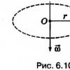
The methods for constructing a statistical model describing a technological process (Figure 6.1) are based on the concept of a "black box". Multiple measurements of input factors are possible for it: x 1, x 2, ..., x k and output parameters: y 1, y 2, ..., y p, according to the results of which dependencies are established:
 In statistical modeling, following the statement of problem (1), the least important factors are eliminated from a large number of input variables that affect the course of the process (2). The input variables selected for further research make up a list of factors x 1, x 2, ..., x k in (6.1), by controlling which one can adjust the output parameters y n... The number of model outputs should also be reduced as much as possible to reduce experimentation and data processing costs.
When developing a statistical model, usually its structure (3) is set arbitrarily, in the form of convenient functions that approximate the experimental data, and then refined based on an assessment of the adequacy of the model.
The most commonly used form is the polynomial form of the model. So, for a quadratic function:
![]() (6.2)
(6.2)
where b 0, b i, b ij, b ii- regression coefficients.
Usually, they first restrict themselves to the simplest linear model, for which in (6.2) b ii = 0, b ij = 0... In the case of its inadequacy, the model is complicated by the introduction of terms that take into account the interaction of factors x i, x j and (or) quadratic terms.
In order to maximize the extraction of information from the conducted experiments and reduce their number, experiments are planned (4) i.e. selection of the number and conditions for conducting experiments necessary and sufficient to solve the set task with a given accuracy.
To build statistical models, two types of experiments are used: passive and active. Passive experiment is carried out in the form of long-term observation of the course of an uncontrolled process, which allows collecting a wide range of data for statistical analysis. IN active experiment there is a possibility of regulating the conditions for conducting experiments. When it is carried out, the most effective is the simultaneous variation of the magnitude of all factors according to a specific plan, which makes it possible to identify the interaction of factors and reduce the number of experiments.
Based on the results of the experiments (5), the regression coefficients (6.2) are calculated and their statistical significance is estimated, which completes the construction of the model (6). The measure of the adequacy of model (7) is variance, i.e. root-mean-square deviation of the calculated values from the experimental ones. The resulting variance is compared with the acceptable variance for the achieved experimental accuracy.
4. Scheme for constructing stochastic models
Building a stochastic model involves developing, evaluating the quality, and investigating the behavior of a system using equations that describe the process under study. For this, initial information is obtained by conducting a special experiment with a real system. At the same time, methods for planning an experiment, processing results, as well as criteria for evaluating the obtained models are used, based on such sections of mathematical statistics as variance, correlation, regression analysis, etc.
Stages of developing a stochastic model:
formulation of the problem
selection of factors and parameters
model type selection
experiment planning
implementation of the experiment according to the plan
building a statistical model
checking the adequacy of the model (related to 8, 9, 2, 3, 4)
model correction
process research with a model (linked to 11)
determination of optimization parameters and constraints
process optimization with a model (linked to 10 and 13)
experimental information of automation equipment
process control with a model (linked to 12)
Combining stages 1 to 9 gives us an information model, from the first to eleventh - an optimization model, combining all points - a management model.
5. Tools for processing models
Using CAE systems, you can perform the following model processing procedures:
imposition of a mesh of finite elements on a 3-dimensional model,
tasks of the heat-stressed state; fluid dynamics problems;
heat and mass transfer tasks;
contact tasks;
kinematic and dynamic calculations, etc.
simulation of complex production systems based on queuing models and Petri nets
Typically, CAE modules provide the ability to color and grayscale images, superimpose the original and deformed parts, visualize liquid and gas flows.
Examples of systems for modeling fields of physical quantities in accordance with FEM: Nastran, Ansys, Cosmos, Nisa, Moldflow.
Examples of systems for modeling dynamic processes at the macro level: Adams and Dyna - in mechanical systems, Spice - in electronic circuits, PA9 - for multidimensional modeling, i.e. for modeling systems, the principles of which are based on the mutual influence of physical processes of various nature.
6. Mathematical modeling. Analytical and simulation models
Mathematical model - a set of mathematical objects (numbers, variables, sets, etc.) and relations between them, which adequately reflects some (essential) properties of the designed technical object. Mathematical models can be geometric, topological, dynamic, logical, etc.
- the adequacy of the representation of the simulated objects;
Adequacy area is an area in the parameter space, within which the model errors remain within acceptable limits.
- economy (computational efficiency)- is determined by the cost of resources,
required for the implementation of the model (costs of computer time, memory used, etc.);
- accuracy - determines the degree of coincidence of the calculated and true results (the degree of correspondence between the estimates of the properties of the same name of the object and the model).
Math modeling- the process of building mathematical models. Includes the following stages: problem statement; building a model and its analysis; development of methods for obtaining design solutions on the model; experimental verification and adjustment of the model and methods.
The quality of the created mathematical models largely depends on the correct formulation of the problem. It is necessary to determine the technical and economic goals of the problem being solved, to collect and analyze all the initial information, to determine the technical limitations. In the process of building models, you should use the methods of systems analysis.
The modeling process, as a rule, is iterative in nature, which provides for the refinement of previous decisions made at the previous stages of model development at each iteration step.
Analytical Models - numerical mathematical models that can be represented in the form of explicit dependences of the output parameters on the parameters of internal and external. Simulation models - numerical algorithmic models displaying the processes in the system in the presence of external influences on the system. Algorithmic models - models in which the relationship between the output, internal and external parameters is set implicitly in the form of a modeling algorithm. Simulation models are often used at the system design level. Simulation modeling is performed by reproducing events that occur simultaneously or sequentially in model time. An example of a simulation model is the use of a Petri net to model a queuing system.
7. Basic principles of building mathematical models
Classical (inductive) approach. The real object to be modeled is divided into separate subsystems, i.e. initial data for modeling are selected and goals are set that reflect individual aspects of the modeling process. For a separate set of initial data, the goal is to simulate a separate side of the system's functioning; on the basis of this goal, a certain component of the future model is formed. A collection of components is combined into a model.
Such a classical approach can be used to create fairly simple models in which separation and mutually independent consideration of individual aspects of the functioning of a real object is possible. Realizes the movement from the particular to the general.
Systems approach. Based on the initial data that are known from the analysis of the external system, those restrictions that are imposed on the system from above or based on the possibilities of its implementation, and on the basis of the goal of functioning, the initial requirements for the system model are formulated. On the basis of these requirements, approximately some subsystems, elements are formed and the most difficult stage of synthesis is carried out - the choice of the components of the system, for which special selection criteria are used. The systems approach also presupposes a certain sequence of model development, which consists in identifying two main stages of design: macro-design and micro-design.
Macro design stage- on the basis of data on the real system and the external environment, a model of the external environment is built, resources and limitations for building a model of the system are identified, a model of the system and criteria are selected that allow assessing the adequacy of the model of a real system. Having constructed a model of the system and a model of the external environment, on the basis of the criterion of the effectiveness of the functioning of the system in the process of modeling, the optimal control strategy is chosen, which makes it possible to realize the possibility of the model to reproduce certain aspects of the functioning of a real system.
Micro-design stage highly depends on the specific type of model chosen. In the case of a simulation model, it is necessary to ensure the creation of information, mathematical, technical and software for the simulation system. At this stage, it is possible to establish the main characteristics of the created model, estimate the time of working with it and the costs of resources to obtain a given quality of conformity of the model to the process of the functioning of the system.  when building it, it is necessary to be guided by a number of principles of a systematic approach:
proportional and sequential progress through the stages and directions of creating a model;
coordination of information, resource, reliability and other characteristics;
the correct ratio of individual levels of the hierarchy in the modeling system;
the integrity of individual isolated stages of model building.
Analysis of the applied methods in mathematical modeling
In mathematical modeling, the solution of differential or integro-differential equations with partial derivatives is performed by numerical methods. These methods are based on discretization of independent variables - their representation by a finite set of values at selected nodal points of the investigated space. These points are considered as nodes of some mesh.
Among the grid methods, two methods are most widely used: the finite difference method (FCD) and the finite element method (FEM). Typically, spatial independent variables are sampled, i. E. use a spatial grid. In this case, the discretization result is a system of ordinary differential equations, which are then reduced to a system of algebraic equations using the boundary conditions.
Let it be necessary to solve the equation LV(z) = f(z)
with given boundary conditions MV(z) = .(z),
where L and M - differential operators, V(z) - phase variable, z= (x 1, x 2, x 3, t) is a vector of independent variables, f(z) and ψ. ( z) are given functions of independent variables.
IN MKR the algebraization of derivatives with respect to spatial coordinates is based on the approximation of derivatives by finite-difference expressions. When using the method, you need to select the grid steps for each coordinate and the type of template. A pattern is understood as a set of nodal points, the values of the variables in which are used to approximate the derivative at one specific point.
FEM is based on the approximation not of the derivatives, but of the solution itself V(z). But since it is unknown, the approximation is performed by expressions with undefined coefficients.
In this case, we are talking about approximations of the solution within finite elements, and taking into account their small sizes, we can talk about using relatively simple approximating expressions (for example, polynomials of low degrees). As a result of the substitution such polynomials into the original differential equation and performing differentiation operations, the values of the phase variables are obtained at the given points.
Polynomial approximation. The use of the methods is associated with the possibility of approximating a smooth function by a polynomial and then using an approximating polynomial to estimate the coordinates of the optimum point. The necessary conditions for the effective implementation of such an approach are unimodality and continuity investigated function. According to the Weierstrass approximation theorem, if a function is continuous in some interval, then it can be approximated with any degree of accuracy by a polynomial of a sufficiently high order. According to the Weierstrass theorem, the quality of the estimates of the optimum point coordinates obtained using the approximating polynomial can be improved in two ways: using a higher order polynomial and decreasing the approximation interval. The simplest form of polynomial interpolation is a quadratic approximation, which is based on the fact that a function that takes a minimum value at an interior point of an interval must be at least quadratic
Discipline "Models and methods of analysis of design solutions" (Kazakov Yu.M.)
Classification of mathematical models.
Abstraction levels of mathematical models.
Requirements for mathematical models.
Scheme for constructing stochastic models.
Model processing tools.
Math modeling. Analytical and simulation models.
Basic principles of building mathematical models.
Analysis of the applied methods in mathematical modeling.
1. Classification of mathematical models
Mathematical model (MM) of a technical object is a collection of mathematical objects (numbers, variables, matrices, sets, etc.) and relations between them, which adequately reflects the properties of a technical object that are of interest to the engineer who develops this object.
By the nature of the display of object properties:
Functional - designed to display physical or informational processes occurring in technical systems during their operation. A typical functional model is a system of equations describing either electrical, thermal, mechanical processes, or information transformation processes.
Structural - displays the structural properties of an object (topological, geometric). . Structural models are most often represented in the form of graphs.
By belonging to the hierarchical level:
Microlevel models - display of physical processes in continuous space and time. The apparatus of equations of mathematical physics is used for modeling. Examples of such equations are partial differential equations.
Macro-level models. Enlargement, detailing of the space on a fundamental basis are used. Functional models at the macrolevel are systems of algebraic or ordinary differential equations; appropriate numerical methods are used to obtain and solve them.
Meta-level models. Enlarged describe the objects under consideration. Mathematical models at the metalevel - systems of ordinary differential equations, systems of logical equations, simulation models of queuing systems.
By the method of obtaining the model:
Theoretical - are built on the basis of studying patterns. In contrast to empirical models, theoretical in most cases are more universal and applicable to a wider range of problems. Theoretical models are linear and non-linear, continuous and discrete, dynamic and statistical.
Empirical
The main requirements for mathematical models in CAD:
the adequacy of the representation of the simulated objects;
Adequacy takes place if the model reflects the specified properties of the object with acceptable accuracy and is assessed by the list of reflected properties and areas of adequacy. Adequacy area is an area in the parameter space, within which the model errors remain within acceptable limits.
economy (computational efficiency)- is determined by the costs of resources required for the implementation of the model (costs of computer time, used memory, etc.);
accuracy- determines the degree of coincidence of the calculated and true results (the degree of correspondence between the estimates of the properties of the same name of the object and the model).
A number of other requirements are imposed on mathematical models:
Computability, i.e. the possibility of manual or computer-assisted study of the qualitative and quantitative laws of the functioning of an object (system).
Modularity, i.e. correspondence of model constructions to the structural components of the object (system)
Algorithmizability, i.e. the possibility of developing an appropriate algorithm and program that implements the mathematical model on a computer.
Visibility, i.e. convenient visual perception of the model.
Table. Classification of mathematical models
|
Classification signs |
Types of mathematical models |
|
1. Belonging to the hierarchical level |
Microlevel models Macro-level models Metalevel models |
|
2. The nature of the displayed properties of the object |
Structural Functional |
|
3. Method of representing object properties |
Analytical Algorithmic Imitation |
|
4. Method of obtaining the model |
Theoretical Empirical |
|
5. Features of the object's behavior |
Deterministic Probabilistic |
Micro-level mathematical models manufacturing processes reflect the physical processes occurring, for example, when cutting metals. They describe processes at the transition level.
Macro-level mathematical models manufacturing process describe technological processes.
Mathematical models at the meta-level of the production process describe technological systems (sections, workshops, the enterprise as a whole).
Structural Mathematical Models are designed to display the structural properties of objects. For example, in CAD TP to represent the structure of the technological process, the ordering of products, structural and logical models are used.
Functional mathematical models are designed to display information, physical, time processes occurring in operating equipment, during the execution of technological processes, etc.
Theoretical mathematical models are created as a result of the study of objects (processes) at a theoretical level.
Empirical mathematical models are created as a result of experiments (studying the external manifestations of the properties of an object by measuring its parameters at the input and output) and processing their results by methods of mathematical statistics.
Deterministic mathematical models describe the behavior of an object from the standpoint of complete certainty in the present and future. Examples of such models: formulas of physical laws, technological processes of processing parts, etc.
Probabilistic mathematical models take into account the influence of random factors on the behavior of the object, i.e. assess its future from the standpoint of the likelihood of certain events.
Analytical models - numerical mathematical models that can be represented in the form of explicit dependences of the output parameters on the parameters of internal and external.
Algorithmic mathematical models express the relationship between the output parameters and the input and internal parameters in the form of an algorithm.
Simulation mathematical models- these are algorithmic models that reflect the development of the process (behavior of the investigated object) in time when specifying external influences on the process (object). For example, these are models of queuing systems given in algorithmic form.
Send your good work in the knowledge base is simple. Use the form below
Students, graduate students, young scientists who use the knowledge base in their studies and work will be very grateful to you.
Posted on http://www.allbest.ru/
1. An example of building a stochastic process model
In the course of a bank's functioning, it is often necessary to solve the problem of choosing a vector of assets, i.e. the bank's investment portfolio, and the uncertain parameters that must be taken into account in this task are primarily associated with the uncertainty of asset prices (securities, real investments, etc.). As an illustration, we can give an example with the formation of a portfolio of government short-term liabilities.
For problems of this class, the fundamental issue is the construction of a model of the stochastic process of price changes, since the researcher of the operation, naturally, has only a finite series of observations of realizations of random variables - prices. Further, one of the approaches to solving this problem is presented, which is being developed at the Computing Center of the Russian Academy of Sciences in connection with the solution of control problems for stochastic Markov processes.
Considered M types of securities, i=1,… , M that are traded on special exchange sessions. The securities are characterized by values - expressed as a percentage of yields during the current session. If a security of the type at the end of the session is bought at the price and sold at the end of the session at the price, then.
Returns are random values formed as follows. The existence of basic returns is assumed - random variables that form a Markov process and are determined by the following formula:
Here, are constants, and are standard normally distributed random variables (i.e., with zero mathematical expectation and unit variance).
where is a certain scale factor equal to (), and is a random variable that has the meaning of a deviation from the base value and is defined similarly:
where - also, standard normally distributed random variables.
It is assumed that some operating party, hereinafter called the operator, for some time manages its capital invested in securities (at any moment in securities of exactly one type), selling them at the end of the current session and immediately buying other securities with the proceeds. Management, selection of purchased securities is performed according to an algorithm that depends on the operator's awareness of the process that forms the yield of securities. We will consider various hypotheses about this awareness and, accordingly, various control algorithms. We will assume that an operation researcher develops and optimizes a control algorithm using the available series of observations of the process, i.e., using information about closing prices at exchange sessions, as well as, possibly, about values at a certain time interval corresponding to sessions with numbers. The purpose of the experiments is to compare the estimates of the expected efficiency of various control algorithms with their theoretical mathematical expectation under conditions when the algorithms are tuned and evaluated on the same series of observations. To estimate the theoretical mathematical expectation, the Monte Carlo method is used by "sweeping" control over a sufficiently large generated series, i.e. by a matrix of dimensions, where the columns correspond to realizations of values and by sessions, and the number is determined by computational capabilities, but provided that the elements of the matrix are at least 10,000. It is necessary that the "polygon" be the same in all experiments. The existing series of observations mimics the generated dimension matrix, where the values in the cells have the same meaning as above. The number and values in this matrix will vary in the future. Matrices of both types are formed by means of a procedure for generating random numbers that simulates the implementation of random variables, and calculating the desired elements of the matrices using these realizations and formulas (1) - (3).
Evaluation of management efficiency over a number of observations is made according to the formula
where is the index of the last session in the series of observations, and is the number of bonds selected by the algorithm at step, i.e. of the type of bonds, in which, according to the algorithm, the operator's capital will be located during the session. In addition, we will also calculate the monthly efficiency. The number 22 roughly corresponds to the number of trading sessions per month.
Computational experiments and analysis of results
Hypotheses
Operator's exact knowledge of future returns.
The index is chosen as. This option gives an upper estimate for all possible control algorithms, even if additional information (taking into account some additional factors) will make it possible to refine the price forecast model.
Random control.
The operator does not know the law of pricing and conducts operations by random choice. Theoretically, in this model, the mathematical expectation of the result of operations is the same as if the operator invested not in one security, but in everything equally. With zero mathematical expectations of values, the mathematical expectation of a value is 1. Calculations based on this hypothesis are useful only in the sense that they allow to some extent check the correctness of the written programs and the generated matrix of values.
Management with accurate knowledge of the profitability model, all its parameters and the observed value .
In this case, the operator at the end of the session, knowing the values for both sessions, and, and in our calculations, using the rows, and, matrices, calculates the mathematical expectations of values by formulas (1) - (3) and selects the paper with the largest of these values of quantities.
where, according to (2),. (6)
Management with knowledge of the structure of the model of returns and the observed value , but unknown coefficients .
We will assume that the investigator of the operation not only does not know the values of the coefficients, but also does not know the number of the previous values of these parameters influencing the formation of values (the memory depth of Markov processes). He also does not know whether the coefficients are the same or different for different values. Consider various options for the researcher's actions - 4.1, 4.2, and 4.3, where the second index denotes the researcher's assumption about the memory depth of processes (the same for and). For example, in case 4.3, the researcher assumes that it is formed according to the equation
An intercept has been added here for completeness. However, this term can be excluded either from substantive considerations or by statistical methods. Therefore, to simplify the calculations, we exclude free terms from consideration when setting the parameters in the future, and formula (7) takes the form:
Depending on whether the researcher assumes the same or different coefficients for different values, we will consider subcases 4.m. 1 - 4.m. 2, m = 1 - 3. In cases 4.m. 1 coefficients will be adjusted according to the observed values for all securities together. In cases 4.m. 2 coefficients are adjusted for each security separately, while the researcher works under the hypothesis that the coefficients are different for different and, for example, in the case of 4.2.2. the values are determined by the modified formula (3)
First way of setting- the classical least squares method. Let's consider it on the example of setting the coefficients for in options 4.3.
According to formula (8),
It is required to find such values of the coefficients in order to minimize the sample variance for realizations on a known series of observations, an array, provided that the mathematical expectation of the values is determined by formula (9).
Hereinafter, the sign "" indicates the realization of a random variable.
The minimum of the quadratic form (10) is attained at a single point at which all partial derivatives are equal to zero. From this we obtain a system of three algebraic linear equations:
the solution of which gives the desired values of the coefficients.
After the coefficients are verified, the choice of controls is carried out in the same way as in case 3.
Comment. In order to facilitate the work on the programs, the procedure for choosing a control, described for hypothesis 3, was adopted, immediately to be written, focusing not on formula (5), but on its modified version in the form
In this case, in the calculations for cases 4.1.m and 4.2.m, m = 1, 2, the excess coefficients are reset to zero.
Second way of setting consists in choosing the values of the parameters so as to maximize the estimate from formula (4). This task is analytically and computationally hopelessly difficult. Therefore, here we can only talk about the methods of some improvement in the value of the criterion relative to the starting point. As a starting point, you can take the values obtained by the least squares method, and then calculate around these values on a grid. In this case, the sequence of actions is as follows. First, the grid is calculated using the parameters (square or cube) with the rest of the parameters fixed. Then, for cases 4.m. 1, the grid is calculated on the parameters, and for cases 4.m. 2 on the parameters with the remaining parameters fixed. In the case of 4.m. 2, then the parameters are also optimized. When all parameters are exhausted by this process, the process is repeated. Repetitions are made until the new cycle gives an improvement in the values of the criterion compared to the previous one. To prevent the number of iterations from being too large, we apply the following technique. Inside each block of calculations on a 2 or 3-dimensional space of parameters, a sufficiently coarse grid is first taken, then, if the best point is on the edge of the grid, then the investigated square (cube) is shifted and the calculation is repeated, if the best point is internal, then a new grid is built around this point with a smaller step, but with the same total number of points, and so some, but a reasonable number of times.
Unobservable control and without taking into account the dependence between the yields of different securities.
This means that the researcher of the operation does not notice the dependence between different securities, does not know anything about the existence and tries to predict the behavior of each paper separately. Consider, as usual, three cases when a researcher models the process of generating returns in the form of a Markov process with depths of 1, 2, and 3:
The coefficients for forecasting the expected profitability are not important, and the coefficients are adjusted in two ways described in paragraph 4. The controls are selected in the same way as it was done above.
Note: As well as for the choice of control, for the least squares method it makes sense to write a single procedure with the maximum number of variables - 3. If the adjustable variables, say, then for the solution of the linear system a formula is written out, which includes only constants, is determined by , and through and. In cases where there are fewer than three variables, the values of the extra variables are set to zero.
Although the calculations are carried out in the same way in different variants, the number of variants is quite large. When the preparation of tools for calculations in all of the above options is difficult, the issue of reducing their number is considered at the expert level.
Unobservable control taking into account the relationship between the yields of different securities.
This series of experiments simulates the manipulations that were performed in the GKO problem. We assume that the researcher knows practically nothing about the mechanism of formation of returns. He has only a number of observations, a matrix. For substantive reasons, he makes an assumption about the interdependence of the current yields of different securities, grouped around a certain basic yield, determined by the state of the market as a whole. Considering the graphs of securities yields from session to session, he makes the assumption that at each moment of time the points, the coordinates of which are the numbers of securities and yields (in reality, these were the terms to maturity of securities and their prices), are grouped near a certain curve (in the case of GKO - parabolas).
Here is the point of intersection of the theoretical line with the ordinate axis (basic yield), and is its slope (which should be equal to 0.05).
Having thus constructed the theoretical straight lines, the researcher of the operation can calculate the values - the deviations of the quantities from their theoretical values.
(Note that here they have a slightly different meaning than in formula (2). There is no dimensional coefficient, and deviations are considered not from the base value, but from the theoretical straight line.)
The next task is to predict values from the values known at the time,. Because the
to predict the values, the researcher needs to enter a hypothesis about the formation of the values, and. According to the matrix, the researcher can establish a significant correlation between the values and. It is possible to accept the hypothesis of a linear relationship between the quantities from:. From meaningful considerations, the coefficient is immediately assumed to be zero, and the least squares method is sought in the form:
Further, as above, they are modeled by means of the Markov process and are described by formulas similar to (1) and (3) with a different number of variables depending on the memory depth of the Markov process in the considered version. (here it is determined not by formula (2), but by formula (16))
Finally, as above, two methods of setting the parameters by the least squares method are implemented, and estimates are made by directly maximizing the criterion.
Experiments
For all the options described, the criterion scores were calculated for different matrices. (matrices with the number of rows 1003, 503, 103 and for each variant of the dimension were implemented about a hundred matrices). Based on the calculation results for each dimension, the mathematical expectation and variance of the values, and their deviation from the values, were estimated for each of the prepared options.
As shown by the first series of computational experiments with a small number of tunable parameters (about 4), the choice of the tuning method does not significantly affect the value of the criterion in the problem.
2. Modeling tool classification
stochastic simulation bank algorithm
The classification of modeling methods and models can be carried out according to the degree of detail of the models, according to the nature of features, according to the scope of application, etc.
Consider one of the most common classifications of models by modeling tools, this aspect is the most important in the analysis of various phenomena and systems.
material in the case when the research is carried out on models, the connection of which with the object under investigation exists objectively, has a material character. Models in this case are built by the researcher or chosen by him from the surrounding world.
By means of modeling, modeling methods are divided into two groups: material methods and methods of ideal modeling. Modeling is called material in the case when the research is carried out on models, the connection of which with the object under investigation exists objectively, has a material character. Models in this case are built by the researcher or chosen by him from the surrounding world. In turn, material modeling can be distinguished: spatial, physical and analog modeling.
In spatial modeling models are used to reproduce or display the spatial properties of the object under study. Models in this case are geometrically similar to objects of study (any models).
Models used in physical modeling are designed to reproduce the dynamics of processes occurring in the object under study. Moreover, the commonality of the processes in the object of research and the model is based on the similarity of their physical nature. This modeling method is widely used in engineering for the design of various types of technical systems. For example, the study of aircraft based on experiments in a wind tunnel.
Analog modeling is associated with the use of material models that have a different physical nature, but described by the same mathematical relations as the object under study. It is based on an analogy in the mathematical description of a model and an object (the study of mechanical vibrations using an electrical system described by the same differential equations, but more convenient in conducting experiments).
In all cases of material modeling, the model is a material reflection of the original object, and the study consists in material impact on the model, that is, in the experiment with the model. Material modeling is by nature an experimental method and is not used in economic research.
Fundamentally different from material modeling perfect simulation based on the ideal, conceivable connection between the object and the model. Ideal modeling methods are widely used in economic research. They can be conditionally divided into two groups: formalized and non-formalized.
IN formalized In modeling, systems of signs or images serve as a model, together with which the rules for their transformation and interpretation are set. If systems of signs are used as models, then modeling is called iconic(drawings, graphs, diagrams, formulas).
An important type of sign modeling is math modeling, based on the fact that different objects and phenomena under study can have the same mathematical description in the form of a set of formulas, equations, the transformation of which is carried out on the basis of the rules of logic and mathematics.
Another form of formalized modeling is figurative, in which the models are built on visual elements (elastic balls, fluid flows, trajectories of motion of bodies). The analysis of figurative models is carried out mentally, therefore, they can be attributed to formalized modeling, when the rules for the interaction of objects used in the model are clearly fixed (for example, in an ideal gas, the collision of two molecules is considered as a collision of balls, and the result of the collision is thought of by everyone in the same way). Models of this type are widely used in physics, they are usually called "thought experiments".
Unformalized modeling. It includes such an analysis of various types of problems, when the model is not formed, and instead of it, some precisely not fixed mental reflection of reality is used, which serves as the basis for reasoning and decision-making. Thus, any reasoning that does not use a formal model can be considered an unformalized modeling, when a thinking individual has a certain image of the object of research, which can be interpreted as an unformalized model of reality.
The study of economic objects for a long time was carried out only on the basis of such vague ideas. At present, the analysis of non-formalized models remains the most common means of economic modeling, namely, any person who makes an economic decision without using mathematical models is forced to be guided by one or another description of the situation based on experience and intuition.
The main disadvantage of this approach is that the solutions may turn out to be of little efficiency or error. For a long time, apparently, these methods will remain the main means of making decisions not only in most ordinary situations, but also in making decisions in the economy.
Posted on Allbest.ru
...Similar documents
Principles and stages of building an autoregressive model, its main advantages. The spectrum of the autoregression process, the formula for finding it. Parameters characterizing the spectral estimate of a random process. The characteristic equation of the autoregressive model.
test, added 11/10/2010
The concept and types of models. Stages of building a mathematical model. Fundamentals of mathematical modeling of the relationship of economic variables. Determination of the parameters of a linear one-way regression equation. Optimization methods of mathematics in economics.
abstract, added 02/11/2011
Investigation of the features of the development and construction of a model of the socio-economic system. Description of the main stages of the imitation process. Experimenting with a simulation model. Organizational aspects of simulation.
abstract, added 06/15/2015
The concept of simulation modeling, its application in economics. Stages of the process of constructing a mathematical model of a complex system, criteria for its adequacy. Discrete Event Modeling. The Monte Carlo method is a type of simulation.
test, added 12/23/2013
Methodological foundations of econometrics. Problems of constructing econometric models. Aims of econometric research. The main stages of econometric modeling. Econometric models of paired linear regression and methods for evaluating their parameters.
test, added 10/17/2014
Stages of building decision trees: the rule of splitting, stopping and cutting. Statement of the problem of multi-step stochastic choice in the subject area. Evaluation of the probability of the implementation of successful and unsuccessful activities in the task, its optimal path.
abstract, added 05/23/2015
Definition, goals and objectives of econometrics. Stages of building a model. Data types for modeling economic processes. Examples, shapes and patterns. Endogenous and exogenous variables. Building the specification of a neoclassical production function.
presentation added 03/18/2014
The main thesis of formalization. Simulation of dynamic processes and simulation of complex biological, technical, social systems. Analysis of object modeling and selection of all its known properties. The choice of the form of the model presentation.
abstract, added 09/09/2010
The main stages of mathematical modeling, classification of models. Modeling economic processes, the main stages of their research. System prerequisites for the formation of a model of a system for managing the marketing activities of a service sector enterprise.
abstract, added 06/21/2010
General diagram of the design process. Formalization of the construction of a mathematical model during optimization. Examples of using one-dimensional search methods. Zero-order multivariate optimization methods. Genetic and natural algorithms.
Series "Economics and Management"
6. Kondratyev N.D. Big business cycles and the theory of foresight. - M .: Economics, 2002.768 p.
7. Kuzyk B.N., Kushlin V.I., Yakovets Yu.V. Forecasting, strategic planning and national programming. M .: Publishing house "Economics", 2008.573 p.
8. Lyasnikov N.V., Dudin M.N. Modernization of the innovative economy in the context of the formation and development of the venture market // Social Sciences. M .: Publishing house "MII Nauka", 2011. No. 1. P. 278-285.
9. Sekerin V.D., Kuznetsova O.S. Development of an innovative project management strategy // Bulletin of the Moscow State Academy of Business Administration. Series: Economics. - 2013. No. 1 (20). - S. 129 - 134.
10. Yakovlev V.M., Senin A.S. There is no alternative to the innovative type of development of the Russian economy // Actual problems of innovative economics. M .: Publishing House "Science"; Institute of Management and Marketing of RAKhN and GS under the President of the Russian Federation, 2012. No. 1 (1).
11. Baranenko S. P., Dudin M. N., Ljasnikov N. V., Busygin KD. Using environmental approach to innovation-oriented development of industrial enterprises // American Journal of Applied Sciences. - 2014. - Vol. 11, No.2, - P. 189-194.
12. Dudin M.N. A systematic approach to determining the modes of interaction of large and small businesses // European Journal of Economic Studies. 2012. Vol. (2), No. 2, P. 84-87.
13. Dudin M.N., Ljasnikov N.V., Kuznecov A.V., Fedorova I. Ju. Innovative Transformation and Transformational Potential of Socio-Economic Systems // Middle East Journal of Scientific Research, 2013. Vol. 17, No. 10. P. 1434-1437.
14. Dudin M.N., Ljasnikov N.V., Pankov S.V., Sepiashvili E.N. Innovative foresight as the method for management of strategic sustainable development of the business structures // World Applied Sciences Journal. - 2013. - Vol. 26, No. 8. - P. 1086-1089.
15. Sekerin V. D., Avramenko S. A., Veselovsky M. Ya., Aleksakhina V. G. B2G Market: The Essence and Statistical Analysis // World Applied Sciences Journal 31 (6): 1104-1108, 2014
Construction of a one-parameter, stochastic model of the production process
Ph.D. Assoc. Mordasov Yu.P.
University of Mechanical Engineering, 8-916-853-13-32, [email protected] hi
Annotation. The author has developed a mathematical, stochastic model of the production process, depending on one parameter. The model was tested. For this, a simulation model of the production, machine-building process has been created, taking into account the influence of random disturbances-failures. Comparison of the results of mathematical and simulation modeling confirms the feasibility of using the mathematical model in practice.
Key words: technological process, mathematical, simulation model, operational control, approbation, random disturbances.
The costs of operational management can be significantly reduced by developing a methodology that allows you to find the optimum between the costs of operational planning and losses that result from the mismatch of planned indicators with the indicators of real production processes. This means finding the optimal signal travel time in the feedback loop. In practice, this means a reduction in the number of calculations of the calendar schedules for launching assembly units into production and, due to this, saving material resources.
The course of the production process in mechanical engineering is of a probabilistic nature. The constant influence of constantly changing factors does not make it possible to predict for a certain perspective (month, quarter) the course of the production process in space and time. In statistical models of scheduling, the state of a part at each specific moment in time should be specified in the form of the corresponding probability (probability distribution) of finding it at different workplaces. At the same time, it is necessary to ensure the determinism of the final result of the enterprise. This, in turn, implies the ability, using deterministic methods, to plan certain periods of time for parts to be in production. However, experience shows that various interrelationships and mutual transitions of real production processes are diverse and numerous. When developing deterministic models, this creates significant difficulties.
An attempt to take into account all the factors influencing the course of production makes the model cumbersome, and it ceases to perform the functions of a planning, accounting and regulation tool.
A simpler method for constructing mathematical models of complex real processes, depending on a large number of different factors, which are difficult or even impossible to take into account, is the construction of stochastic models. In this case, when analyzing the principles of functioning of a real system or when observing its individual characteristics, probability distribution functions are constructed for some parameters. In the presence of high statistical stability of the quantitative characteristics of the process and their low variance, the results obtained using the constructed model are in good agreement with the indicators of the functioning of the real system.
The main prerequisites for building statistical models of economic processes are:
Excessive complexity and associated economic inefficiency of the corresponding deterministic model;
Large deviations of the theoretical indicators obtained as a result of the experiment on the model from the indicators of actually functioning objects.
Therefore, it is desirable to have a simple mathematical apparatus describing the influence of stochastic disturbances on the global characteristics of the production process (commodity output, volume of work in progress, etc.). That is, to build a mathematical model of the production process, depending on a small number of parameters and reflecting the total influence of many factors of a different nature on the course of the production process. The main task that a researcher should set himself when building a model is not a passive observation of the parameters of a real system, but the construction of a model that, for any deviation under the influence of disturbances, would bring the parameters of the displayed processes to a given mode. That is, under the action of any random factor in the system, a process should be established that converges to a planned solution. Currently, in automated control systems, this function is mainly assigned to a person who is one of the links in the feedback chain in the management of production processes.
Let's turn to the analysis of a real production process. Usually the duration of the planning period (the frequency of issuing plans to shops) is selected based on the traditionally established calendar time intervals: shift, day, five days, etc. They are guided mainly by practical considerations. The minimum duration of the planning period is determined by the operational capabilities of the planned bodies. If the production and dispatch department of the enterprise copes with the issuance of adjusted shift tasks to the shops, then the calculation is made for each shift (that is, the costs associated with the calculation and analysis of planned tasks are made every shift).
To determine the numerical characteristics of the probability distribution of random
Series "Economics and Management" of troubles, we will build a probabilistic model of a real technological process of manufacturing one assembly unit. Here and hereinafter, the technological process of manufacturing an assembly unit means a sequence of operations (work on the manufacture of these parts or assemblies), documented in the technology. Each technological operation of manufacturing products in accordance with the technological route can be performed only after the previous one. Consequently, the technological process of manufacturing an assembly unit is a sequence of events-operations. Under the influence of various stochastic reasons, the duration of an individual operation may change. In some cases, the operation may not be completed during the duration of this shift task. Obviously, these events can be decomposed into elementary components: performance and non-performance of individual operations, which can also be associated with the probability of performance and non-performance.
For a specific technological process, the probability of performing a sequence consisting of K operations can be expressed by the following formula:
PC5 = k) = (1-pk + 1) PG = 1P1, (1)
where: Р1 - the probability of performing the 1st operation, taken separately; d - the number of the operation in order in the technological process.
This formula can be used to determine the stochastic characteristics of a specific planning period, when the range of products launched into production and the list of works that must be performed in a given planning period, as well as their stochastic characteristics, which are determined empirically, are known. In practice, the listed requirements are satisfied only by some types of mass production with high statistical stability of characteristics.
The likelihood of performing one particular operation depends not only on external factors, but also on the specific nature of the work performed and on the type of assembly unit.
To determine the parameters of the above formula, even with a relatively small set of assembly units, with small changes in the nomenclature of products, a significant amount of experimental data is required, which causes significant material and organizational costs and makes this method of determining the probability of uninterrupted production of products hardly applicable.
Let us examine the resulting model for the possibility of its simplification. The initial value of the analysis is the probability of failure-free execution of one operation of the technological process of manufacturing products. In real production conditions, the probabilities of performing operations of each type are different. For a specific technological process, this probability depends on:
From the type of operation being performed;
From a specific assembly unit;
From products manufactured in parallel;
From external factors.
Let us analyze the influence of fluctuations in the probability of performing one operation on the enlarged characteristics of the production process of manufacturing products (volume of commodity output, volume of work in progress, etc.), determined using this model. The aim of the study is to analyze the possibility of replacing different probabilities of performing one operation with the mean value in the model.
The combined influence of all the above factors is taken into account when calculating the geometric mean probability of performing one operation of the averaged technological process. Analysis of modern production shows that it fluctuates insignificantly: practically in the range of 0.9 - 1.0.
A clear illustration of how low the probability of performing one operation
walkie talkie corresponds to a value of 0.9, is the following abstract example. Let's say you want to make ten parts. Technological processes for the manufacture of each of them contain ten operations. The probability of performing each operation is 0.9. Let's find the probabilities of lagging behind the schedule for a different number of technological processes.
A random event, when a specific technological process of manufacturing an assembly unit lags behind the schedule, corresponds to underperforming at least one operation in this process. It is the opposite of an event: all operations are performed without failure. Its probability is 1 - 0.910 = 0.65. Since delays are independent events, the Bernoulli probability distribution can be used to determine the likelihood of delays for different numbers of processes. The calculation results are shown in Table 1.
Table 1
Calculation of the probabilities of lagging behind the schedule of technological processes
k C ^ o0.35k0.651O-k Sum
The table shows that with a probability of 0.92, five technological processes, that is, half, will lag behind the schedule. The mathematical expectation of the number of technological processes lagging behind the schedule will be 6.5. This means that on average 6.5 assembly units out of 10 will lag behind the schedule. That is, on average, from 3 to 4 parts will be produced without failures. The author is not aware of examples of such a low level of labor organization in real production. The considered example clearly shows that the imposed restriction on the value of the probability of performing one operation without failures does not contradict practice. All of the above requirements are met by the production processes of mechanical assembly shops of machine-building production.
Thus, in order to determine the stochastic characteristics of production processes, it is proposed to construct a probability distribution of the operational execution of one technological process, which expresses the probability of performing a sequence of technological operations of manufacturing an assembly unit in terms of the geometric mean probability of performing one operation. The probability of performing K operations in this case will be equal to the product of the probabilities of performing each operation, multiplied by the probability of non-fulfillment of the rest of the technological process, which coincides with the probability of non-fulfillment of the (K + T) -th operation. This fact is explained by the fact that if any operation fails, then the following operations cannot be executed. The last record differs from the others, as it expresses the probability of complete passage without failures of the entire technological process. The probability of performing the K first operations of the technological process is unambiguously related to the probability of non-execution of the remaining operations. Thus, the probability distribution is as follows:
PJ = 0) = p ° (1-p),
P (g = 1) = p1 (1-p), (2)
P (^ = 1) = p1 (1-p),
P (t = u-1) = pn "1 (1 - p), P (t = n) = pn,
where: ^ is a random variable, the number of operations performed;
p is the geometric mean probability of performing one operation, n is the number of operations in the technological process.
The validity of the application of the obtained one-parameter probability distribution is intuitively visible from the following reasoning. Suppose that we have calculated the geometric mean of the probability of performing one 1 operation on a sample consisting of n elements, where n is large enough.
p = USCHT7P7 = tl | n] t = 1p!), (3)
where: Iу - the number of operations with the same probability of execution; ] - index of a group of operations that have the same probability of execution; t is the number of groups consisting of operations that have the same probability of execution;
^ = - - the relative frequency of occurrence of operations with the probability of execution p ^.
According to the law of large numbers, with an unlimited number of operations, the relative frequency of occurrence in a sequence of operations with certain stochastic characteristics tends in probability to the probability of this event. Whence it follows that
for two sufficiently large samples =, which means:
where: т1, т2 - the number of groups in the first and second samples, respectively;
1 *, I2 - the number of elements in the group of the first and second samples, respectively.
Hence, it can be seen that if the parameter is calculated for a large number of tests, then it will be close to the parameter P, calculated for this sufficiently large sample.
Attention should be paid to the different closeness to the true value of the probabilities of performing a different number of operations in the technological process. In all elements of the distribution, except for the last one, there is a factor (I - P). Since the value of the parameter P is in the range of 0.9 - 1.0, the multiplier (I - P) ranges from 0 - 0.1. This factor corresponds to the factor (I - p;) in the original model. Experience shows that this match for a particular probability can cause an error of up to 300%. However, in practice, they are usually interested not in the probabilities of performing any number of operations, but in the probability of complete execution without disruptions of the technological process. This probability does not contain a factor (I - P), and, therefore, its deviation from the actual value is small (practically no more than 3%). For economic tasks, this is quite high accuracy.
The probability distribution of a random variable constructed in this way is a stochastic dynamic model of the manufacturing process of an assembly unit. Time participates in it implicitly, as the duration of one operation. The model makes it possible to determine the probability that after a certain period of time (the corresponding number of operations) the production process of manufacturing an assembly unit will not be interrupted. For mechanical assembly shops of mechanical engineering production, the average number of operations in one technological process is quite large (15 - 80). If we consider this number as basic and assume that, on average, in the manufacture of one assembly unit, a small set of enlarged types of work (turning, locksmith, milling, etc.) is used,
then the obtained distribution can be successfully applied to assess the influence of stochastic disturbances on the course of the production process.
The author carried out a simulation experiment based on this principle. To generate a sequence of pseudo-random values uniformly distributed over the interval 0.9 - 1.0, the pseudo-random number sensor described in the work was used. The experiment software is written in the algorithmic language COBOL.
In the experiment, products of generated random variables are formed that simulate the real probabilities of complete execution of a specific technological process. They are compared with the probability of performing the technological process, obtained using the geometric mean, which was calculated for a sequence of random numbers of the same distribution. The geometric mean is raised to a power equal to the number of factors in the product. A percentage difference is calculated between these two results. The experiment is repeated for a different number of multipliers in the products and the number of numbers for which the geometric mean is calculated. A fragment of the experimental results is shown in Table 2.
table 2
Results of the simulation experiment:
n is the degree of the geometric mean; k - the degree of the product
n to Work Deviation to Work Deviation to Work Deviation
10 1 0,9680 0% 7 0,7200 3% 13 0,6277 -7%
10 19 0,4620 -1% 25 0,3577 -1% 31 0,2453 2%
10 37 0,2004 6% 43 0,1333 4% 49 0,0888 6%
10 55 0,0598 8% 61 0,0475 5% 67 0,0376 2%
10 73 0,0277 1% 79 0,0196 9% 85 0,0143 2%
10 91 0,0094 9% 97 0,0058 0%
13 7 0,7200 8% 13 0,6277 0% 19 0,4620 0%
13 25 0,3577 5% 31 0,2453 6% 37 0,2004 4%
13 43 0,1333 3% 49 0,0888 8% 55 0,0598 8%
13 61 0,0475 2% 67 0,0376 8% 73 0,0277 2%
13 79 0,0196 1% 85 0,0143 5% 91 0,0094 5%
16 1 0,9680 0% 7 0,7200 9%
16 13 0,6277 2% 19 0,4620 3% 25 0,3577 0%
16 31 0,2453 2% 37 0,2004 2% 43 0,1333 5%
16 49 0,0888 4% 55 0,0598 0% 61 0,0475 7%
16 67 0,0376 5% 73 0,0277 5% 79 0,0196 2%
16 85 0,0143 4% 91 0,0094 0% 97 0,0058 4%
19 4 0,8157 4% 10 0,6591 1% 16 0,5795 -9%
19 22 0,4373 -5% 28 0,2814 5% 34 0,2256 3%
19 40 0,1591 6% 46 0,1118 1% 52 0,0757 3%
19 58 0,0529 4% 64 0,0418 3% 70 0,0330 2%
19 76 0,0241 6% 82 0,0160 1% 88 0,0117 8%
19 94 0,0075 7% 100 0,0048 3%
22 10 0,6591 4% 16 0,5795 -4% 22 0,4373 0%
22 28 0,2814 5% 34 0,2256 5% 40 0,1591 1%
22 46 0,1118 1% 52 0,0757 0% 58 0,0529 8%
22 64 0,0418 1% 70 0,0330 3% 76 0,0241 5%
22 82 0,0160 4% 88 0,0117 2% 94 0,0075 5%
22 100 0,0048 1%
25 4 0,8157 3% 10 0,6591 0%
25 16 0,5795 0% 72 0,4373 -7% 28 0,2814 2%
25 34 0,2256 9% 40 0,1591 1% 46 0,1118 4%
25 52 0,0757 5% 58 0,0529 4% 64 0,0418 2%
25 70 0,0330 0% 76 0,0241 2% 82 0,0160 4%
28 4 0,8157 2% 10 0,6591 -2% 16 0,5795 -5%
28 22 0,4373 -3% 28 0,2814 2% 34 0,2256 -1%
28 40 0,1591 6% 46 0,1118 6% 52 0,0757 1%
28 58 0,0529 4% 64 0,041 8 9% 70 0,0330 5%
28 70 0,0241 2% 82 0,0160 3% 88 0,0117 1%
28 94 0,0075 100 0,0048 5%
31 10 0,6591 -3% 16 0,5795 -5% 22 0,4373 -4%
31 28 0,2814 0% 34 0,2256 -3% 40 0,1591 4%
31 46 0,1118 3% 52 0,0757 7% 58 0,0529 9%
31 64 0,0418 4% 70 0,0330 0% 76 0,0241 6%
31 82 0,0160 6% 88 0,0117 2% 94 0,0075 5%
When setting up this simulation experiment, the goal was to investigate the possibility of obtaining, using the probability distribution (2), one of the enlarged statistical characteristics of the production process - the probability of performing without failures one technological process of manufacturing an assembly unit, consisting of K operations. For a specific technological process, this probability is equal to the product of the probabilities of performing all its operations. As the simulation experiment shows, its relative deviations from the probability obtained using the developed probabilistic model do not exceed 9%.
Since a more inconvenient than real probability distribution was used in the simulation experiment, the practical discrepancies will be even smaller. Deviations are observed both in the direction of decrease and in the direction of exceeding the value obtained from the averaged characteristics. This fact suggests that if we consider the deviation of the probability of failure-free execution of not a single technological process, but several, then it will be much less. Obviously, it will be the smaller, the more technological processes will be considered. Thus, the simulation experiment shows a good agreement between the probability of the production process without disruptions in the production of products with the probability obtained using a one-parameter mathematical model.
In addition, simulation experiments were carried out:
To study the statistical convergence of the probability distribution parameter estimates;
To study the statistical stability of the mathematical expectation of the number of operations performed without failures;
For the analysis of methods for determining the duration of the minimum planning period and assessing the discrepancy between the planned and real indicators of the production process, with a mismatch in time between the planned and production periods.
Experiments have shown good agreement between theoretical data obtained based on the application of techniques and empirical data obtained using simulation on
Series "Economics and Management"
Computer for real production processes.
Based on the use of the constructed mathematical model, the author has developed three specific methods for increasing the efficiency of operational management. For their approbation, separate simulation experiments were carried out.
1. Methodology for determining the rational volume of production targets for the planning period.
2. Methodology for determining the most effective duration of the operational planning period.
3. Estimation of mismatch in case of mismatch in time of planned and production periods.
Literature
1. Mordasov Yu.P. Determination of the duration of the minimum operational planning period under the conditions of the action of random disturbances / Economic-mathematical and simulation modeling with the use of computers. - M: MIU them. S. Ordzhonikidze, 1984.
2. Naylor T. Machine simulation experiments with models of economic systems. -M: Mir, 1975.
The transition from concentration to diversification is an effective way of developing the economy of small and medium-sized businesses
prof. Kozlenko N. N. University of Mechanical Engineering
Annotation. This article examines the problem of choosing the most effective development of Russian small and medium-sized businesses by moving from a concentration strategy to a diversification strategy. The issues of expediency of diversification, its advantages, criteria for choosing the path of diversification are considered, the classification of diversification strategies is given.
Key words: small and medium-sized businesses; diversification; strategic fit; competitive advantages.
An active change in the parameters of the macroenvironment (changing market conditions, the emergence of new competitors in related industries, an increase in the level of competition in general) often leads to non-fulfillment of the planned strategic plans of small and medium-sized businesses, losses of financial and economic stability of enterprises due to a significant gap between the objective conditions of small enterprises and the level of technology to manage them.
The main conditions for economic stability and the ability to maintain competitive advantages are the ability of the management system to respond in a timely manner and change internal production processes (change the assortment taking into account diversification, rebuild production and technological processes, change the structure of the organization, use innovative marketing and management tools).
The study of the practice of Russian small and medium-sized enterprises of industrial type and service maintenance revealed the following features and basic cause-and-effect relationships regarding the current trend of the transition of small enterprises from concentration to diversification.
Most small and medium-sized businesses start out as small, single-business businesses serving local or regional markets. At the beginning of its activity, the range of products of such a company is very limited, its capital base is weak, and its competitive position is vulnerable. Typically, the strategy of these companies focuses on increasing sales and market share, as well as