With a large number of observations or with a large numerical value, the option is used
a simplified way of calculating the arithmetic mean - the way of moments.
M = A + iSap
where M is the arithmetic mean; A - conditional average; i - interval between groups option;
S - summation sign .; a - conditional deviation of each option from the conditional average;
p is the frequency of occurrence of the variant; n is the number of observations.
An example of calculating the arithmetic mean by the method of moments (average body weight
boys aged 18)
| V (n in kg) | R | a (V-A) | a. R |
| +2 | +4 | ||
| +1 | +3 | ||
| M about = 62 | |||
| -1 | -6 | ||
| -2 | -8 | ||
| -3 | -3 | ||
| n = 25 | Sar = - 10kg |
Stages of calculating the average by the method of moments:
2) define "a" - the conditional deviation of the options from the conditional average, for this we subtract the conditional average from each option: a = V - A, (for example, a = 64 - 62 = +2, etc.).
3) we multiply the conditional deviation "a" by the frequency "p" of each option and get the product a p;
4) find the sum Sа. p = - 10kg
5) calculate the arithmetic mean by the method of moments:
M = A + i SaP= 62 - 1 × 0.4 = 61.6kg
Thus, we can conclude that in the studied group of young men, the average body weight is
The arithmetic mean by itself does not say anything about the variation series from which
it has been calculated. Its typicality (reliability) is influenced by the homogeneity of the considered
material and the oscillation of the series.
Example: given two variational series of the same number of observations, in which
presents the data of measurements of the head circumference of children aged 1 to 2 years
Having the same number of observations and the same arithmetic means (M = 46 cm), the series
have differences in distribution internally. So the options for the first row deviate generally from
the arithmetic mean with a lower value than the variants of the second row, which gives
the possibility of assuming that the arithmetic mean (46 cm) is more typical for the first
row than for the second.
In statistics, to characterize the diversity of the variation series, they use the average
standard deviation(s)
There are two ways to calculate the standard deviation: arithmetic mean
way and way of moments. With the arithmetic mean method of calculation, the formula is used:
where d is the true deviation of each option from the true mean M. The formula is used for
a small number of observations (n<30)
Formula for determining s by the method of moments:

where a is the conditional deviation of the options from the conditional average;
The moment of the second degree, and the moment of the first degree, squared.
It has been theoretically and practically proven that if, with a large number of observations, to the average
arithmetic add and subtract 1s (M ± 1s) from it, then within the obtained values
there will be 68.3% of all variants of the variation series. If the arithmetic mean
add and subtract 2s (M ± 2s), then 95.5% will be within the obtained values
all option. М ± 3s includes 99.7% of all variants of the variation series.
Based on this position, you can check the typicality of the arithmetic mean for
the variation series from which it was calculated. To do this, you need to average
add arithmetic and subtract three times s (M ± 3s) from it. If within the obtained limits
the given variation series fits, then the arithmetic mean is typical, i.e. she
expresses the basic pattern of the series and can be used.
This provision is widely used in the development of various standards (clothing,
shoes, school furniture, etc.).
Diversity degree features in the variation series can be estimated by coefficient
variations(the ratio of the standard deviation to the arithmetic mean,
multiplied by 100%)
With v = s x 100
With C v less than 10%, there is a weak diversity, with C v 10-20% - average, and with more than 20% -
strong variety of attribute.
Assessment of the reliability of the results of statistical research
As we said, the most reliable results can be obtained when using
continuous method i.e. when studying the general population.
Meanwhile, the study of the general population is associated with significant laboriousness.
Therefore, in biomedical research, as a rule, selective
observation. In order that the data obtained in the study of the sample population can be
was transferred to the general population, it is necessary to assess the reliability
results of statistical research. The sample population may not be enough
fully represent the general population, therefore, sample observations are always
accompanied by a representativeness error. The size of the average error (m) can be judged
how much the found sample average differs from the general average
the aggregate. A small error indicates the proximity of these indicators, a large error is such
does not give confidence.
The value of the mean error of the arithmetic mean is influenced by the following two circumstances.
First, the homogeneity of the collected material: the less the scattering of the variant around
its mean, the smaller the error of representativeness. Second, the number of observations:
the average error will be the smaller, the larger the number of observations.
The average error of the arithmetic mean is calculated using the following formula:
The average error (error of representativeness) for relative values is determined by
formula:
where m p is the average error of the indicator;
p - indicator in% or in% o
q - (100 -p), (1000 -p)
n is the total number of observations
289 patients left the hospital, 12 of them died.
Relative value (mortality rate) p = (12: 289) x100 = 4.1%; q = 100 -p =
100-4.1 = 95.9, whence
m p = ± ![]()
Thus, the relative value in the repeated study will correspond to
Confidence limits is the maximum and minimum value within which
for a given degree of probability of an error-free forecast, the relative
indicator or average in the population
The confidence limits of the relative value in the general population are determined by
P gene = P select ± tm m
The confidence limits of the arithmetic mean in the general population are determined by the formula:
M gene = M select ± tm m
where P gene and M gene are the values of the relative and average values obtained for the general
the aggregate.
R select and M select - the values of the relative and average values obtained for the sample population.
m р and m m - error of representativeness for mean and relative values.
t - reliability criterion.
It was found that if t = 1, the reliability does not exceed 68%; if t = 2 -95%; if t = 3- 99%
In medical and biological research, it is considered sufficient if the criterion
reliability t ³ 2 (confidence 95%)
To find the criterion t for the number of observations £ 30, it is necessary to use a special
table
With a decrease in the magnitude of the representativeness error, the confidence limits decrease.
average and relative values, i.e. the results of the study are refined, approaching
corresponding values of the general population. If the error of representativeness
large, then they get large confidence limits, which may contradict
logical assessment of the desired value in the general population. Confidence limits
also depend on the degree of probability of an error-free forecast chosen by the researcher. At
a high degree of probability of an error-free forecast the range of confidence limits
Most often, the arithmetic mean is used to characterize the variation series.
There are three types of arithmetic mean: simple, weighted and calculated by the method of moments. The arithmetic mean, which is calculated in a variation series, where each option occurs only 1 time is called arithmetic mean simple (Table 4) It is determined by the formula:
where M is the arithmetic mean,
V - variant of the studied trait,
n is the number of observations.
If in the investigated row one or more options are repeated several times, then calculate weighted arithmetic mean (Table 2) when the weight of each variant is taken into account depending on the frequency of its occurrence. The calculation of such an average is carried out according to the formula:
where M is the weighted arithmetic mean;
∑ - sum sign;
V - options (numerical values of the studied attribute);
P is the frequency with which the same variant of the feature occurs, i.e. the amount of the variant with the given value of the characteristic;
n is the number of observations, i.e., the sum of all frequencies or the total number of all variants (∑p).
Table 4
(Simple arithmetic mean calculation)
| NUMBER OF STUDENTS (p) | |
| ∑V = 691 | n = 9 |
| M = bpm. |
Example: when determining the average heart rate of students before the exam, you should first calculate ∑ V * p, and then the average value M = = 76.9 beats / min. (Table 5).
Often, with a large number of observations, a grouped variational (or divided into equal intervals) series is used to calculate the weighted arithmetic mean. Such a series of variations should be continuous, the options arranged in a certain order (increasing or decreasing) follow each other.
Table 5
Determining the average heart rate of male students before the exam
(Calculation of the weighted arithmetic mean)
| PULSE FOR MEN STUDENTS (V) | NUMBER OF STUDENTS (p) | V * p |
| ∑p = n = 26∑V * p = 2000 M = = 76.9 bpm. |
When grouping the variation series, it should be borne in mind that the interval is chosen by the researcher, the size of the interval depends on the goal and objectives of the study.
The number of groups in a grouped variation series is determined depending on the number of observations. With the number of observations from 31 to 100, it is recommended to have 5-6 groups, from 101 to 300 - from 6 to 8 groups, from 300 to 1000 observations, you can use from 10 to 15 groups ... The calculation of the interval (i) is carried out according to the formula: i =,
Vmax - maximum value of options,
Vmin is the minimum value of the options.
The calculation of the weighted average in the grouped row (or interval row requires the determination of the middle of the interval, which is calculated as the semi-summary values of the group. (Table 3). The calculation of the average value is carried out according to the formula: M = = = 176.7 cm. (Table 6).
Table 6
(Calculate the weighted arithmetic mean in a grouped row)
| CENTRAL GROUP OPTION (V 1), SEE | NUMBER OF STUDENTS (p) | V 1 ∙ p | |
| 162 = 167 = 172 = 177 = 182 187 | |||
| ∑p = n = 212 ∑ V 1 ∙ p = 37469 M = = = 176.74 cm. |
In cases where the options are represented by large numbers (for example, the body weight of newborns in grams) and there is a number of observations expressed in hundreds or thousands of cases, the weighted arithmetic mean can be calculated by the method of moments (Table 7) using the formula:
where A is a conventionally taken average value (most often Mo is taken as a conditional average);
∑ - sum sign;
α - deviation of each option in intervals from the conditional average =
p is the frequency (the number of times with which the same variant of the feature occurs).
αp is the product of the deviation (α) by the frequency (p);
n is the number of observations, i.e. the sum of all frequencies or the total number of all variants (∑p).
i is the value of the interval = (Vmax is the maximum value of the options, Vmin is the minimum value of the options).
Thus, the weighted average calculated by the method of moments was 176.74 cm, which practically coincided with the calculations of the average by the usual method - 176.7 cm. However, when calculating the average by the method of moments, simple numbers are used, the calculation is less cumbersome, which greatly facilitates and speeds up the calculations.
The arithmetic mean (weighted average) has a number of properties, which are used in some cases to simplify the calculation of the average and obtain an approximate value.
1. The arithmetic mean takes the middle position in a strictly symmetrical variation series (M = M 0 = M e).
2. The arithmetic mean has an abstract character and is a generalizing value that reveals a pattern.
3. The algebraic sum of deviations of all variants from the mean is equal to zero: ∑ (V - M) = 0. This property is used to calculate the mean by the method of moments.
Table 7
Determination of the average height of male students 20-22 years old
(Methodology for calculating the arithmetic mean by the method of moments, i = 5)
| GROWTH OF MEN STUDENTS (V) CM. | CENTRAL GROUP VERSION (V 1), SEE | NUMBER OF STUDENTS (p) | α = | a ∙ p | |
| 160-164 165-169 170-174 175-179 180-184 185-189 | ∑p = n = 212 | -3 -2 -1 +1 +2 | -12 -42 -47 +54 +36 ∑a ∙ p = -11 | ||
| M = 177 + | |||||
Properties of the arithmetic mean. Calculation of the arithmetic mean by the "moments" method
To reduce the complexity of calculations, the basic properties of the average arithm are used:
- 1. If all variants of the averaged attribute increase / decrease by a constant value A, then the arithmetic mean will increase / decrease accordingly.
- 2. If all the variants of the characteristic being determined are increased / decreased by n-times, then the average arithm will increase / decrease by n-times.
- 3. If all the frequencies of the averaged attribute are increased / decreased by a constant number of times, then the average arithm will remain unchanged.
- 18. Average harmonic simple and weighted
Harmonic mean - used when statistical information does not contain data on weights for individual variants of the population, but the products of the values of the varying attribute by the corresponding weights are known.
The general formula for the harmonic weighted average is as follows:
x - the value of the variable feature,
w is the product of the value of the varying feature by its weight (xf)
For example, three batches of product A were purchased at different prices (20, 25 and 40 rubles). The total cost of the first batch was 2000 rubles, the second batch was 5000 rubles, and the third batch was 6000 rubles. It is required to determine the average unit price of A.
The average price is determined as the quotient of dividing the total cost by the total amount of purchased goods. Using the harmonic mean, we get the desired result:

In the event that the total volume of phenomena, i.e. the products of feature values by their weights are equal, then the simple harmonic mean is applied:
x - individual values of the characteristic (variants),
n is the total number of options.
Example. Two cars traveled the same path: one at a speed of 60 km / h, and the other at 80 km / h. We take the length of the path that each car has traveled as a unit. Then the average speed will be:

The harmonic mean has a more complex construction than the arithmetic mean. The harmonic mean is used for calculations when not the aggregate units - the carriers of the feature - are used as weights, but the product of these units by the feature values (i.e., m = Xf). The average harmonic downtime should be resorted to in cases of determining, for example, the average cost of labor, time, materials per unit of production, per one part for two (three, four, etc.) enterprises, workers engaged in the manufacture of the same type of product , the same part, product.
Methods for calculating the arithmetic mean (simple and weighted arithmetic mean, by the method of moments)
We determine the average values:
Fashion (Mo) = 11, because this variant occurs most often in the variation series (p = 6).
Median (Me) is the ordinal number of the variants occupying the middle position = 23, this place in the variation series is occupied by the variant equal to 11. The arithmetic mean (M) allows the most complete characterization of the average level of the trait under study. To calculate the arithmetic mean, two methods are used: the arithmetic mean and the moments method.
If the frequency of occurrence of each variant in the variation series is equal to 1, then the arithmetic simple mean is calculated using the arithmetic mean method: M =.
If the frequency of occurrence of a variant in the variation series differs from 1, then the weighted arithmetic mean is calculated using the arithmetic mean method:
By the method of moments: A - conditional average,
M = A + = 11 + = 10.4 d = V-A, A = Mo = 11
If the number of variants in the variation series is more than 30, then a grouped series is built. Building a grouped row:
1) determination of Vmin and Vmax Vmin = 3, Vmax = 20;
2) determination of the number of groups (according to the table);
3) calculating the interval between groups i = 3;
4) determination of the beginning and end of the groups;
5) determination of the frequency of the variant of each group (table 2).
table 2
Method for constructing a grouped row
|
Duration treatment in days |
|||||||
|
n = 45 p = 480 p = 30 2 p = 766 |
The advantage of the grouped variation series is that the researcher does not work with every option, but only with the options that are the average for each group. This makes it much easier to calculate the average.
The magnitude of a particular feature is not the same for all members of the population, despite its relative homogeneity. This feature of the statistical population characterizes one of the group properties of the general population - variety of trait... For example, let's take a group of 12 year old boys and measure their height. After the calculations, the average level of this trait will be 153 cm. But the average characterizes the overall measure of the trait under study. Among boys of this age, there are boys whose height is 165 cm or 141 cm. The more boys have a height other than 153 cm, the greater the diversity of this feature in the statistical population.
Statistics allows you to characterize this property by the following criteria:
limit (lim),
amplitude (Amp),
standard deviation ( y) ,
coefficient of variation (Cv).
Limit (lim) is determined by the extreme values of the variant in the variation series:
lim = V min / V max
Amplitude (Amp) - difference of extreme options:
Amp = V max -V min
These values take into account only the diversity of the extreme variants and do not allow obtaining information about the diversity of the trait in aggregate, taking into account its internal structure. Therefore, these criteria can be used to roughly characterize the diversity, especially with a small number of observations (n<30).
variation series medical statistics
Variational range (or range of variation) - this is the difference between the maximum and minimum values of the characteristic:
In our example, the range of variation in the shift production of workers is: in the first brigade R = 105-95 = 10 children, in the second brigade R = 125-75 = 50 children. (5 times more). This suggests that the output of the 1st brigade is more "stable", but the second brigade has more reserves for the growth of output, because if all workers reach the maximum output for this brigade, it can produce 3 * 125 = 375 parts, and in the 1st brigade only 105 * 3 = 315 parts.
If the extreme values of the trait are not typical for the population, then the quartile or decile ranges are used. The quartile range RQ = Q3-Q1 covers 50% of the population, the decile range of the first RD1 = D9-D1 covers 80% of the data, the second decile range of RD2 = D8-D2 is 60%.
The disadvantage of the indicator of the variation range is, but that its value does not reflect all the fluctuations of the trait.
The simplest generalizing indicator that reflects all fluctuations in a feature is mean linear deviation, which is the arithmetic mean of the absolute deviations of individual options from their mean:
,
for grouped data ![]() ,
,
where xi is the value of a feature in a discrete row or the middle of an interval in an interval distribution.
In the above formulas, the differences in the numerator are taken modulo, otherwise, according to the property of the arithmetic mean, the numerator will always be zero. Therefore, the average linear deviation in statistical practice is rarely used, only in those cases when the summation of indicators without taking into account the sign makes economic sense. With its help, for example, the composition of employees, the profitability of production, and the turnover of foreign trade are analyzed.
Feature variance Is the mean square of the deviations of the variant from their mean value:
simple variance ![]() ,
,
weighted variance  .
.
The formula for calculating variance can be simplified:
Thus, the variance is equal to the difference between the mean of the squares of the variant and the square of the mean of the variant of the population:  .
.
However, due to the summation of the squares of the deviations, the variance gives a distorted idea of the deviations, therefore, the average is calculated on the basis standard deviation, which shows how much, on average, specific variants of a feature deviate from their average value. Calculated by taking the square root of the variance:
for ungrouped data  ,
,
for the variation series 
The smaller the variance and standard deviation, the more homogeneous the population, the more reliable (typical) the mean will be.
The mean linear and standard deviation are named numbers, that is, they are expressed in the units of measurement of the attribute, are identical in content and close in value.
It is recommended to calculate the absolute indicators of variation using tables.
Table 3 - Calculation of the characteristics of the variation (using the example of the period of data on the shift production of the work crew)
Number of workers |
The middle of the interval, |
Calculated values |
|||||
Total: |
|||||||
Average shift production of workers: ![]()
Average linear deviation: ![]()
Dispersion of production: 
The standard deviation of the output of individual workers from the average output:
.
1 Calculation of variance by the method of moments
Calculating variances involves cumbersome calculations (especially if the average is expressed as a large number with several decimal places). Calculations can be simplified by using a simplified formula and dispersion properties.
The dispersion has the following properties:
- if all the values of the attribute are reduced or increased by the same value A, then the variance will not decrease from this:
 ,
,
 then or
Using the properties of the variance and first decreasing all the variants of the population by the value A, and then dividing by the value of the interval h, we obtain the formula for calculating the variance in the variational series with equal intervals way of moments: ,
,
where is the variance calculated by the method of moments;
h is the value of the interval of the variation series;
- new (converted) values option;
A - constant value, which is used as the middle of the interval with the highest frequency; or the variant with the highest frequency;  - square of the moment of the first order;
- moment of the second order.
Let's calculate the variance by the method of moments based on the data on the shift production of the workers of the brigade.
Table 4 - Calculation of variance by the method of moments
Groups of workers for development, pcs. |
Number of workers |
The middle of the interval, |
Calculated values |
||
Calculation procedure:


- we calculate the variance:
2 Calculation of the variance of an alternative feature
Among the features studied by statistics, there are those that are characterized by only two mutually exclusive values. These are alternative signs. They are given, respectively, two quantitative meanings: options 1 and 0. Frequency of options 1, which is denoted by p, is the proportion of units with this feature. The difference 1-p = q is a frequency of options 0. Thus,
xi |
|
The arithmetic mean of the alternative feature ![]() , since p + q = 1.
, since p + q = 1.
Variance of an alternative feature
since 1-p = q
Thus, the variance of an alternative feature is equal to the product of the fraction of units with this feature and the fraction of units that do not have this feature.
If the values 1 and 0 occur equally often, i.e. p = q, the variance reaches its maximum pq = 0.25.
The variance of an alternative characteristic is used in sample surveys, for example, product quality.
3 Intergroup variance. Variance addition rule
Variance, unlike other characteristics of variation, is an additive quantity. That is, in the aggregate, which is divided into groups by factor NS , performance trait variance y can be decomposed into variance in each group (intragroup) and variance between groups (intergroup). Then, along with the study of the variation of the trait for the entire population as a whole, it becomes possible to study the variation in each group, as well as between these groups.
Total variance measures the variation of a trait at in the aggregate under the influence of all factors that caused this variation (deviations). It is equal to the mean square of the deviations of individual values of the attribute at from the total average and can be calculated as a simple or weighted variance.
Intergroup variance characterizes the variation of the effective trait at caused by the influence of the sign factor NS, which is the basis of the grouping. It characterizes the variation of group means and is equal to the mean square of deviations of group means from the total mean:  ,
,
where is the arithmetic mean of the i-th group;
- the number of units in the i-th group (frequency of the i-th group);
- the total average of the population.
Intra-group variance reflects a random variation, that is, that part of the variation that is caused by the influence of unaccounted factors and does not depend on the attribute-factor underlying the grouping. It characterizes the variation of individual values relative to group means, is equal to the mean square of deviations of individual values of the attribute at within a group from the arithmetic mean of this group (group mean) and is calculated as a simple or weighted variance for each group: ![]() or
or ![]() ,
,
where is the number of units in the group.
Based on the intragroup variances for each group, it is possible to determine total mean of intragroup variances:
.
The relationship between the three variances is called variance addition rules, according to which the total variance is equal to the sum of the intergroup variance and the average of the intragroup variances:
Example... When studying the influence of the wage category (qualification) of workers on the level of their labor productivity, the following data were obtained.
Table 5 - Distribution of workers by average hourly production.
№ p / p |
Workers of the 4th category |
Workers of the 5th category |
|||||
Production |
Production |
||||||
1 |
7 |
7-10=-3 |
9 |
1 |
14 |
14-15=-1 |
1 |
In this example, the workers are divided into two groups according to the factor. NS- qualifications, which is characterized by their rank. The productive sign - development - varies both under its influence (intergroup variation) and due to other random factors (intragroup variation). The challenge is to measure these variations using three variances: total, between-group and within-group. The empirical coefficient of determination shows the proportion of variation of the effective trait at under the influence of a factor NS... The rest of the total variation at caused by a change in other factors.
In the example, the empirical coefficient of determination is: ![]() or 66.7%,
or 66.7%,
This means that 66.7% of the variation in labor productivity of workers is due to differences in qualifications, and 33.3% - the influence of other factors.
Empirical correlation relation shows the tightness of the relationship between grouping and effective indicators. Calculated as the square root of the empirical coefficient of determination:
The empirical correlation ratio, like and, can take values from 0 to 1.
If there is no connection, then = 0. In this case = 0, that is, the group means are equal to each other and there is no intergroup variation. This means that the grouping sign is that the factor does not affect the formation of the general variation.
If the connection is functional, then = 1. In this case, the variance of the group means is equal to the total variance (), that is, there is no intra-group variation. This means that the grouping attribute completely determines the variation of the studied productive attribute.
The closer the value of the correlation ratio is to one, the closer, closer to the functional dependence, the relationship between the signs.
For a qualitative assessment of the tightness of the relationship between the signs, the Chaddock ratios are used.
In the example ![]() , which indicates a close relationship between the productivity of workers and their qualifications.
, which indicates a close relationship between the productivity of workers and their qualifications.