Trigonometric series Definition. A function f (x) defined on an unbounded set D is called periodic if there exists a number T Φ 0 such that for each x ∈ D the condition is satisfied. The smallest of such numbers T is called the period of the function f (x). Example 1. A function defined on an interval is periodic, since there is a number T = 2 * φ O such that the condition is satisfied for all x. Thus, the sin x function has a period T = 2g. The same applies to the function Example 2. The function defined on the set D of numbers is periodic, since there is a number T Φ 0, namely, T = such that for x 6 D we have Definition. Functional series of the form ao Fourier series Trigonometric series Orthogonality of a trigonometric system Trigonometric Fourier series Sufficient conditions for the expansion of a function in a Fourier series are called trigonometric series, and the constants a0, a „, bn (n = 1, 2, ...) are called the coefficients of trigonometric series (1 ). The partial sums Sn (g) of the trigonometric series (1) are linear combinations of functions from a system of functions called the trigonometric system. Since the members of this series are periodic functions with period 2π-, then in the case of convergence of series (I) its sum S (x) will be a periodic function with period T = 2mm: Definition. Expanding a periodic function f (x) with a period T = 2n in a trigonometric series (1) means finding a converging trigonometric series, the sum of which is equal to the function f (x). ... Orthogonality of a trigonometric system Definition. Functions f (x) and d (x), continuous on the segment [a, 6], are called orthogonal on this segment, if the condition is satisfied. For example, the functions are orthogonal on the segment [-1,1], since Definition. A finite or infinite system of functions integrable on the segment [a, b] is called an orthogonal system on the segment [a, 6) if for any numbers of type such that m Φ n, the equality holds. Theorem 1. The trigonometric system is orthogonal on the segment For any the whole η Φ 0 we have Using the well-known trigonometry formulas for any natural numbers m and n, m Φ n, we find: Finally, by virtue of the formula for any integers, we obtain the Trigonometric Fourier series Let us set ourselves the task of calculating the coefficients of the trigonometric series (1), knowing the function Theorem 2. Suppose that equality holds for all values of x, and the series on the right-hand side of the equality converges uniformly on the interval [-3r, x]. Then the formulas are valid. The uniform convergence of series (1) implies the continuity, and hence the integrability of the function f (x). Therefore, equalities (2) make sense. Moreover, series (1) can be term-by-term integrated. We have whence and follows the first of formulas (2) for n = 0. Now we multiply both sides of equality (1) by the function cos mi, where m is an arbitrary natural number: Series (3), like series (1), converges uniformly. Therefore, it can be integrated term by term. All integrals on the right-hand side, except for one, which is obtained for n = m, are equal to zero due to the orthogonality of the trigonometric system. Therefore, whence Similarly, multiplying both sides of equality (1) by sinmx and integrating from -m to m, we obtain whence Let there be given an arbitrary periodic function f (x) of period 2 *, integrable on the interval *]. Whether it can be represented as a sum of some converging trigonometric series is not known in advance. However, using formulas (2), it is possible to calculate the constants a „and bn. Definition. The trigonometric series of the coefficients oq, an, bn of which are defined through the function f (x) by the formulas Fourier series Trigonometric series Orthogonality of the trigonometric system Trigonometric Fourier series Sufficient conditions for the expansion of a function in a Fourier series is called the trigonometric Fourier series of the function f (x), and , bnt determined by these formulas are called the Fourier coefficients of the function f (x). Each function f (x) integrable on the interval [-π, -k] can be associated with its Fourier series, that is, trigonometric series, the coefficients of which are determined by formulas (2). However, if nothing is required of the function f (x) except integrability on the interval [-π *, n], then the correspondence sign in the last relation, generally speaking, cannot be replaced by an equal sign. Comment. It is often required to expand in a trigonometric series the function f (x), which is defined only on the interval (- *, n \ and, therefore, is not periodic. Since in formulas (2) for the Fourier coefficients the integrals are calculated over the interval *], then for such function can also be written a trigonometric Fourier series.However, if we continue the function f (x) periodically on the entire Ox axis, then we obtain a function F (x), periodic with period 2n, coinciding with f (x) on the interval (-ir, k):. This function F (x) is called periodically. The sale of the function f (x). In this case, the function F (x) does not have an unambiguous definition at the points x = ± n, ± 3dr, ± 5nr, .... Series The Fourier series for the function F (x) is identical to the Fourier series for the function f (x). Moreover, if the Fourier series for the function f (x) converges to it, then its sum, being a periodic function, gives a periodic continuation of the function f (x) from the segment | -jt, n \ to the entire Ox axis. In this sense, talking about the Fourier series for the function f (x) defined on the interval (-π-, jt | is equivalent to talking about the Fourier series for the function F (x), which is a periodic continuation of the function f (x) to the whole It follows that the criteria for the convergence of Fourier series are sufficient to formulate for periodic functions. § 4. Sufficient conditions for the expansion of a function in a Fourier series We give a sufficient criterion for the convergence of a Fourier series, that is, we formulate conditions on a given function under which the Fourier series converges, and we will find out how the sum of this series behaves in this case.It is important to emphasize that although the class of piecewise monotone functions presented below is rather wide, functions for which the Fourier series converges are not exhausted by it. Definition. Function f ( x) is called piecewise monotone on the segment [a, 6] if this segment can be divided by a finite number of points into intervals, on each of which f (x) is monotone, that is, either does not decrease or does not increase (see Fig. . one). Example 1. The function is piecewise monotonic on the interval (-oo, oo), since this interval can be divided into two intervals (-su, 0) and (0, + oo), on the first of which it decreases (and therefore, does not increase), and on the second it increases (and therefore does not decrease). Example 2. The function is piecewise monotone on the segment [-zr, jt |, since this segment can be divided into two intervals on the first of which cos i increases from -I to +1, and on the second it decreases from. Theorem 3. A function f (x), piecewise monotone and bounded on an interval (a, b], can only have discontinuity points of the first kind on it. Let, for example, be a discontinuity point of the function f (x). Then, by the boundedness of the function f (x) and monotonicity on both sides of the point c, there exist finite one-sided limits This means that the point c is a discontinuity point of the first kind (Fig. 2) Theorem 4. If a periodic function f (x) with period 2nr is piecewise monotone and is bounded on the segment [-t, m), then its Fourier series converges at each point x of this segment, and the sum of this series satisfies the equalities: Prmmer3. The function f (z) of period 2jt, defined on the interval (- *, *) by the equality (Fig. 3), satisfies the conditions of the theorem. Therefore, it can be expanded in a Fourier series. We find the Fourier coefficients for it: The Fourier series for this function has the form Example 4. Expand the function in a Fourier series (Fig. 4) on the interval This function satisfies the conditions of the theorem. Find the Fourier coefficients. Using the additivity property of a definite integral, we will have Fourier series Trigonometric series Orthogonality of a trigonometric system Trigonometric Fourier series Sufficient conditions for the expansion of a function in a Fourier series That is, at the points x = -x and x = x, which are discontinuity points of the first kind, we will have a Remark. If we put x = 0 in the found Fourier series, then we get whence
Hölder's condition. We say that the function $ f (x) $ satisfies the Hölder condition at the point $ x_0 $ if there exist one-sided finite limits $ f (x_0 \ pm 0) $ and such numbers $ \ delta> 0 $, $ \ alpha \ in ( 0,1] $ and $ c_0> 0 $, that for all $ t \ in (0, \ delta) $ the following inequalities hold: $ | f (x_0 + t) -f (x_0 + 0) | \ leq c_0t ^ ( \ alpha) $, $ | f (x_0-t) -f (x_0-0) | \ leq c_0t ^ (\ alpha) $.
Dirichlet's formula. The transformed Dirichlet formula is called a formula of the form:
$$ S_n (x_0) = \ frac (1) (\ pi) \ int \ limits_ (0) ^ (\ pi) (f (x_0 + t) + f (x_0-t)) D_n (t) dt \ quad (1), $$ where $ D_n (t) = \ frac (1) (2) + \ cos t + \ ldots + \ cos nt = \ frac (\ sin (n + \ frac (1) (2)) t) (2 \ sin \ frac (t) (2)) (2) $ -.
Using formulas $ (1) $ and $ (2) $, we write down the partial sum of the Fourier series in the following form:
$$ S_n (x_0) = \ frac (1) (\ pi) \ int \ limits_ (0) ^ (\ pi) \ frac (f (x_0 + t) + f (x_0-t)) (2 \ sin \ frac (t) (2)) \ sin \ left (n + \ frac (1) (2) \ right) t dt $$
$$ \ Rightarrow \ lim \ limits_ (n \ to \ infty) S_n (x_0) - \ frac (1) (\ pi) \ int \ limits_ (0) ^ (\ pi) \ frac (f (x_0 + t) + f (x_0-t)) (2 \ sin \ frac (t) (2)) \ cdot \\ \ cdot \ sin \ left (n + \ frac (1) (2) \ right) t dt = 0 \ quad (3) $$
For $ f \ equiv \ frac (1) (2) $ the formula $ (3) $ takes the following form: $$ \ lim \ limits_ (n \ to \ infty) \ frac (1) (\ delta) \ frac (\ sin (n + \ frac (1) (2)) t) (2 \ sin \ frac (t) (2)) dt = \ frac (1) (2), 0
Convergence of the Fourier series at a point
Theorem. Let $ f (x) $ - $ 2 \ pi $ -periodic function absolutely integrable on $ [- \ pi, \ pi] $ and satisfy the Hölder condition at the point $ x_0 $. Then the Fourier series of the function $ f (x) $ at the point $ x_0 $ converges to the number $$ \ frac (f (x_0 + 0) + f (x_0-0)) (2). $$
If at the point $ x_0 $ the function $ f (x) $ is continuous, then at this point the sum of the series is equal to $ f (x_0) $.
Proof
Since the function $ f (x) $ satisfies the Hölder condition at the point $ x_0 $, then for $ \ alpha> 0 $ and $ 0< t$ $ < \delta$ выполнены неравенства (1), (2).
For a given $ \ delta> 0 $, we write the equalities of $ (3) $ and $ (4) $. Multiplying $ (4) $ by $ f (x_0 + 0) + f (x_0-0) $ and subtracting the result from $ (3) $, we get $$ \ lim \ limits_ (n \ to \ infty) (S_n (x_0) - \ frac (f (x_0 + 0) + f (x_0-0)) (2) - \\ - \ frac (1) (\ pi) \ int \ limits_ (0) ^ (\ delta) \ frac (f (x_0 + t) + f (x_0-t) -f (x_0 + 0) -f (x_0-0)) (2 \ sin \ frac (t) (2)) \ cdot \\ \ cdot \ sin \ left (n + \ frac (1) (2) \ right) t \, dt) = 0. \ quad (5) $$
It follows from Hölder's condition that the function $$ \ Phi (t) = \ frac (f (x_0 + t) + f (x_0-t) -f (x_0 + 0) -f (x_0-0)) (2 \ sin \ frac (t) (2)). $$ is absolutely integrable on the segment $$. Indeed, applying Hölder's inequality, we obtain that the function $ \ Phi (t) $ satisfies the following inequality: $ | \ Phi (t) | \ leq \ frac (2c_0t ^ (\ alpha)) (\ frac (2) (\ pi) t) = \ pi c_0t ^ (\ alpha - 1) (6) $, where $ \ alpha \ in (0,1 ] $.
By virtue of the comparison criterion for improper integrals, it follows from inequality $ (6) $ that $ \ Phi (t) $ is absolutely integrable on $. $
By Riemann's lemma $$ \ lim \ limits_ (n \ to \ infty) \ int \ limits_ (0) ^ (\ delta) \ Phi (t) \ sin \ left (n + \ frac (1) (2) \ right) t \ cdot dt = 0. $$
From the formula $ (5) $ it now follows that $$ \ lim \ limits_ (n \ to \ infty) S_n (x_0) = \ frac (f (x_0 + 0) + f (x_0-0)) (2). $$
[collapse]
Corollary 1. If the $ 2 \ pi $ -periodic and absolutely integrable on $ [- \ pi, \ pi] $ function $ f (x) $ has a derivative at the point $ x_0 $, then its Fourier series converges at this point to $ f (x_0) $.
Corollary 2. If the $ 2 \ pi $ -periodic and absolutely integrable on $ [- \ pi, \ pi] $ function $ f (x) $ has both one-sided derivatives at the point $ x_0 $, then its Fourier series converges at this point to $ \ frac (f (x_0 + 0) + f (x_0-0)) (2). $
Corollary 3. If the $ 2 \ pi $ -periodic and absolutely integrable on $ [- \ pi, \ pi] $ function $ f (x) $ satisfies the Hölder condition at the points $ - \ pi $ and $ \ pi $, then by virtue of the periodicity the sum of the series The Fourier at the points $ - \ pi $ and $ \ pi $ equals $$ \ frac (f (\ pi-0) + f (- \ pi + 0)) (2). $$
Dini's sign
Definition. Let $ f (x) $ be a $ 2 \ pi $ -periodic function, the point $ x_0 $ will be a regular point of the function $ f (x) $ if
- 1) there are finite left and right limits $ \ lim \ limits_ (x \ to x_0 + 0) f (x) = \ lim \ limits_ (x \ to x_0-0) f (x) = f (x_0 + 0) = f (x_0-0), $
- 2) $ f (x_0) = \ frac (f (x_0 + 0) + f (x_0-0)) (2). $
Theorem. Let $ f (x) $ - $ 2 \ pi $ -periodic absolutely integrable on $ [- \ pi, \ pi] $ function and point $ x_0 \ in \ mathbb (R) $ be a regular point of function $ f (x) $ ... Let the function $ f (x) $ satisfy the Dini conditions at the point $ x_0 $: there exist improper integrals $$ \ int \ limits_ (0) ^ (h) \ frac (| f (x_0 + t) -f (x_0 + 0) |) (t) dt, \\ \ int \ limits_ (0) ^ (h) \ frac (| f (x_0-t) -f (x_0-0) |) (t) dt, $$
then the Fourier series of the function $ f (x) $ at the point $ x_0 $ has the sum $ f (x_0) $, that is, $$ \ lim \ limits_ (n \ to \ infty) S_n (x_0) = f (x_0) = \ frac (f (x_0 + 0) + f (x_0-0)) (2). $$
Proof
For the partial sum $ S_n (x) $ of the Fourier series, there is an integral representation $ (1) $. And by virtue of the equality $ \ frac (2) (\ pi) \ int \ limits_ (0) ^ (\ pi) D_n (t) \, dt = 1, $
$$ f (x_0) = \ frac (1) (\ pi) \ int \ limits_ (0) ^ (\ pi) f (x_0 + 0) + f (x_0-0) D_n (t) \, dt $$
Then we have $$ S_n (x_0) -f (x_0) = \ frac (1) (\ pi) \ int \ limits_ (0) ^ (\ pi) (f (x_0 + t) -f (x_0 + 0)) D_n (t) \, dt + $$ $$ + \ frac (1) (\ pi) \ int \ limits_ (0) ^ (\ pi) (f (x_0-t) -f (x_0-0)) D_n (t) \, dt. \ quad (7) $$
Obviously, the theorem will be proved if we prove that both integrals in the formula $ (7) $ have limits for $ n \ to \ infty $ equal to $ 0 $. Consider the first integral: $$ I_n (x_0) = \ int \ limits_ (0) ^ (\ pi) (f (x_0 + t) -f (x_0 + 0)) D_n (t) dt. $$
At the point $ x_0 $, the Dini condition is satisfied: the improper integral $$ \ int \ limits_ (0) ^ (h) \ frac (| f (x_0 + t) -f (x_0 + 0) |) (t) \, dt . $$
Therefore, for any $ \ varepsilon> 0 $, there is a $ \ delta \ in (0, h) $ such that $$ \ int \ limits_ (0) ^ (\ delta) \ frac (\ left | f (x_0 + t) -f (x_0 + 0) \ right |) (t) dt
For the chosen $ \ varepsilon> 0 $ and $ \ delta> 0 $, the integral $ I_n (x_0) $ can be represented as $ I_n (x_0) = A_n (x_0) + B_n (x_0) $, where
$$ A_n (x_0) = \ int \ limits_ (0) ^ (\ delta) (f (x_0 + t) -f (x_0 + 0)) D_n (t) dt, $$ $$ B_n (x_0) = \ int \ limits _ (\ delta) ^ (\ pi) (f (x_0 + t) -f (x_0 + 0)) D_n (t) dt. $$
Consider first $ A_n (x_0) $. Using the estimate $ \ left | D_n (t) \ right |
for all $ t \ in (0, \ delta) $.
Therefore $$ A_n (x_0) \ leq \ frac (\ pi) (2) \ int \ limits_ (0) ^ (\ delta) \ frac (| f (x_0 + t) -f (x_0 + 0) |) ( t) dt
Let us proceed to estimating the integral $ B_n (x_0) $ as $ n \ to \ infty $. To do this, we introduce the function $$ \ Phi (t) = \ left \ (\ begin (matrix)
\ frac (f (x_0 + t) -f (x_0 + 0)) (2 \ sin \ frac (t) (2)), 0
$$ B_n (x_0) = \ int \ limits _ (- \ pi) ^ (\ pi) \ Phi (t) \ sin \ left (n + \ frac (1) (2) \ right) t \, dt. $$ We get that $ \ lim \ limits_ (n \ to \ infty) B_n (x_0) = 0 $, which means that for the previously chosen arbitrary $ \ varepsilon> 0 $ there exists $ N $ such that for all $ n> N $ the inequality holds $ | I_n (x_0) | \ leq | A_n (x_0) | + | B_n (x_0) |
It is proved in exactly the same way that the second integral of the formula $ (7) $ has a zero limit as $ n \ to \ infty $.
[collapse]
Consequence If the $ 2 \ pi $ periodic function $ f (x) $ is piecewise differentiable on $ [- \ pi, \ pi] $, then its Fourier series at any point $ x \ in [- \ pi, \ pi] $ converges to the number $$ \ frac (f (x_0 + 0) + f (x_0-0)) (2). $$
On the segment $ [- \ pi, \ pi] $ find the trigonometric Fourier series of the function $ f (x) = \ left \ (\ begin (matrix)
1, x \ in (0, \ pi), \\ -1, x \ in (- \ pi, 0),
\\ 0, x = 0.
\ end (matrix) \ right. $
Investigate the convergence of the resulting series.
Continuing periodically $ f (x) $ on the whole real axis, we get the function $ \ widetilde (f) (x) $, the graph of which is shown in the figure.
Since the function $ f (x) $ is odd, then $$ a_k = \ frac (1) (\ pi) \ int \ limits _ (- \ pi) ^ (\ pi) f (x) \ cos kx dx = 0; $$
$$ b_k = \ frac (1) (\ pi) \ int \ limits _ (- \ pi) ^ (\ pi) f (x) \ sin kx \, dx = $$ $$ = \ frac (2) (\ pi) \ int \ limits_ (0) ^ (\ pi) f (x) \ sin kx \, dx = $$ $$ = - \ frac (2) (\ pi k) (1- \ cos k \ pi) $$
$$ b_ (2n) = 0, b_ (2n + 1) = \ frac (4) (\ pi (2n + 1)). $$
Therefore, $ \ tilde (f) (x) \ sim \ frac (4) (\ pi) \ sum_ (n = 0) ^ (\ infty) \ frac (\ sin (2n + 1) x) (2n + 1 ). $
Since $ (f) "(x) $ exists for $ x \ neq k \ pi $, then $ \ tilde (f) (x) = \ frac (4) (\ pi) \ sum_ (n = 0) ^ (\ infty) \ frac (\ sin (2n + 1) x) (2n + 1) $, $ x \ neq k \ pi $, $ k \ in \ mathbb (Z). $
At the points $ x = k \ pi $, $ k \ in \ mathbb (Z) $, the function $ \ widetilde (f) (x) $ is undefined, and the sum of the Fourier series is zero.
Setting $ x = \ frac (\ pi) (2) $, we obtain the equality $ 1 - \ frac (1) (3) + \ frac (1) (5) - \ ldots + \ frac ((- 1) ^ n) (2n + 1) + \ ldots = \ frac (\ pi) (4) $.
[collapse]
Find the Fourier series of the following $ 2 \ pi $ -periodic and absolutely integrable on $ [- \ pi, \ pi] $ function:
$ f (x) = - \ ln |
\ sin \ frac (x) (2) | $, $ x \ neq 2k \ pi $, $ k \ in \ mathbb (Z) $, and investigate the convergence of the resulting series.
Since $ (f) "(x) $ exists for $ x \ neq 2k \ pi $, the Fourier series of the function $ f (x) $ will converge at all points $ x \ neq 2k \ pi $ to the value of the function. Obviously that $ f (x) $ is an even function and therefore its Fourier series expansion must contain cosines. Let us find the coefficient $ a_0 $. We have $$ \ pi a_0 = -2 \ int \ limits_ (0) ^ (\ pi) \ ln \ sin \ frac (x) (2) dx = $$ $$ = -2 \ int \ limits_ (0) ^ (\ frac (\ pi) (2)) \ ln \ sin \ frac (x) (2) dx \, - \, 2 \ int \ limits _ (\ frac (\ pi) (2)) ^ (\ pi) \ ln \ sin \ frac (x) (2) dx = $$ $$ = -2 \ int \ limits_ (0) ^ (\ frac (\ pi) (2)) \ ln \ sin \ frac (x) (2) dx \, - \, 2 \ int \ limits_ (0) ^ (\ frac (\ pi ) (2)) \ ln \ cos \ frac (x) (2) dx = $$ $$ = -2 \ int \ limits_ (0) ^ (\ frac (\ pi) (2)) \ ln (\ frac (1) (2) \ sin x) dx = $$ $$ = \ pi \ ln 2 \, - \, 2 \ int \ limits_ (0) ^ (\ frac (\ pi) (2)) \ ln \ sin x dx = $$ $$ = \ pi \ ln 2 \, - \, \ int \ limits_ (0) ^ (\ pi) \ ln \ sin \ frac (t) (2) dt = \ pi \ ln 2 + \ frac (\ pi a_0) (2), $$ whence $ a_0 = \ pi \ ln 2 $.
Let us now find $ a_n $ for $ n \ neq 0 $. We have $$ \ pi a_n = -2 \ int \ limits_ (0) ^ (\ pi) \ cos nx \ ln \ sin \ frac (x) (2) dx = $$ = \ int \ limits_ (0) ^ (\ pi) \ frac (\ sin (n + \ frac (1) (2)) x + \ sin (n- \ frac (1) (2)) x) (2n \ sin \ frac (x) (2) ) dx = $$ $$ = \ frac (1) (2n) \ int \ limits _ (- \ pi) ^ (\ pi) \ begin (bmatrix)
D_n (x) + D_ (n-1) (x) \\ \ end (bmatrix) dx. $$
Here $ D_n (x) $ is the Dirichlet kernel defined by formula (2) and we obtain that $ \ pi a_n = \ frac (\ pi) (n) $ and, therefore, $ a_n = \ frac (1) (n) $. Thus, $$ - \ ln |
\ sin \ frac (x) (2) | = \ ln 2 + \ sum_ (n = 1) ^ (\ infty) \ frac (\ cos nx) (n), x \ neq 2k \ pi, k \ in \ mathbb (Z). $$
[collapse]
Literature
- Lysenko Z.M., lecture notes on mathematical analysis, 2015-2016.
- Ter-Krikorov A.M. and Shabunin M.I. The course of mathematical analysis, pp. 581-587
- Demidovich B.P., Collection of tasks and exercises on mathematical analysis, edition 13, revised, CheRo Publishing House, 1997, pp. 259-267
Time limit: 0
Navigation (job numbers only)
0 of 5 questions completed
Information
Test on the material of this topic:
You have already taken the test before. You cannot start it again.
The test is loading ...
You must login or register in order to start the test.
You must complete the following tests to start this one:
results
Correct answers: 0 out of 5
Your time:
Time is over
You scored 0 out of 0 points (0)
Your result has been recorded on the leaderboard
- With the answer
- Marked as viewed
Task 1 of 5
1 .
Points: 1If the $ 2 \ pi $ -periodic and absolutely integrable on $ [- \ pi, \ pi] $ function $ f (x) $ has a derivative at the point $ x_0 $, then to what will its Fourier series converge at this point?
Question 2 of 5
2 .
Points: 1If all the conditions of the Dini test are satisfied, then to what number does the Fourier series of the function $ f $ converge at the point $ x_0 $?
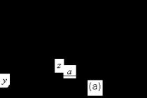
Navier's solution is only suitable for calculating plates hinged along the contour. More general is Levy's solution... It allows you to calculate a plate pivotally supported on two parallel sides, with arbitrary boundary conditions on each of the other two sides.
In the rectangular plate shown in Fig. 5.11, (a), the edges parallel to the axis are pivotally supported. y... The boundary conditions at these edges are
 |
Rice. 5.11
It is obvious that each term of the infinite trigonometric series
https://pandia.ru/text/78/068/images/image004_89.gif "width =" 99 "height =" 49 ">; second partial derivatives of the deflection function
 (5.45)
at x = 0 and x = a also equal to zero, since they contain https://pandia.ru/text/78/068/images/image006_60.gif "width =" 279 "height =" 201 src = "> (5.46)
Substitution of (5.46) into (5.18) gives
Multiplying both sides of the resulting equation by, integrating in the range from 0 to a and remembering that
 ,
,
we obtain for the definition of the function Ym such a linear differential equation with constant coefficients
 . (5.48)
If to shorten the record we denote
equation (5.48) takes the form
 . (5.50)
The general solution of the inhomogeneous equation (5.50), as is known from the course of differential equations, has the form
Ym(y) = jm (y)+ Fm(y), (5.51)
where jm (y) Is a particular solution of the inhomogeneous equation (5.50); its form depends on the right-hand side of equation (5.50), i.e., in fact, on the type of load q (x, y);
Fm(y)= Am shamy + Bm chamy + y(Cm shamy + Dm chamy), (5.52)
general solution of homogeneous equation
Four arbitrary constants Am,INm ,Cm and Dm must be determined from four conditions for fixing the edges of the plate parallel to the axis, applied to the plate constant q (x, y) = q the right-hand side of equation (5.50) takes the form
https://pandia.ru/text/78/068/images/image014_29.gif "width =" 324 "height =" 55 src = ">. (5.55)
Since the right-hand side of equation (5.55) is constant, the left-hand side is also constant; therefore all derivatives jm (y) are equal to zero, and
 , (5.56)
 , (5.57)
where indicated:.
Consider a plate pinched along edges parallel to the axis NS(Figure 5.11, (c)).
Edge conditions y = ± b/2
 . (5.59)
Due to the symmetry of the deflection of the plate relative to the axis Ox, in the general solution (5.52) only the terms containing even functions should be retained. Since sh amy- the function is odd, and сh am y- even and, at the accepted position of the axis Oh, y sh amy- even, in at ch am y Is odd, then the general integral (5.51) in the case under consideration can be represented as follows
 . (5.60)
Since in (5.44) does not depend on the value of the argument y, the second pair of boundary conditions (5.58), (5.59) can be written in the form:
Ym = 0, (5.61)
Y¢ m = = 0. (5.62)
amBm sh amy + Cm(sh amy + yam ch amy)
From (5.60) - (5.63) it follows
https://pandia.ru/text/78/068/images/image025_20.gif "width =" 364 "height =" 55 src = ">. (5.65)
Multiplying equation (5.64) by, and equation (5..gif "width =" 191 "height =" 79 src = ">. (5.66)
Substitution of (5.66) into equation (5.64) makes it possible to obtain Bm
https://pandia.ru/text/78/068/images/image030_13.gif "width =" 511 "height =" 103 ">. (5.68)
With this expression, the functions Ym. , formula (5.44) for determining the deflection function takes the form
 (5.69)
The series (5.69) converges quickly. For example, for a square plate in its center, that is, for x =a/2, y = 0
 (5.70)
Keeping in (5.70) only one term of the series, i.e., taking  , we get the deflection value overestimated by less than 2.47%. Considering that p 5 =
306.02, find Variation "href =" / text / category / variatciya / "rel =" bookmark "> V. Ritz's variational method is based on the Lagrange variational principle formulated in section 2.
, we get the deflection value overestimated by less than 2.47%. Considering that p 5 =
306.02, find Variation "href =" / text / category / variatciya / "rel =" bookmark "> V. Ritz's variational method is based on the Lagrange variational principle formulated in section 2.
Let us consider this method in relation to the problem of plate bending. Imagine the curved surface of the plate in the form of a row
 , (5.71)
where fi(x, y) continuous coordinate functions, each of which must satisfy kinematic boundary conditions; Ci- unknown parameters determined from the Lagrange equation. This equation
 (5.72)
leads to a system of n algebraic equations with respect to parameters Ci.
In the general case, the deformation energy of the plate consists of bending U and membrane U m parts
 , (5.73)
 , (5.74)
where Mx.,My. ,Mxy- bending forces; NNS., Ny. , Nxy- membrane forces. The part of the energy corresponding to the transverse forces is small and can be neglected.
If u, v and w- components of the actual movement, px. , py and pz- components of the intensity of the surface load, Ri- concentrated force, D i the corresponding linear displacement, Mj- concentrated moment, qj- the angle of rotation corresponding to it (Fig.5.12), then the potential energy of external forces can be represented as follows:
If the edges of the plate allow displacement, then the edge forces vn. , mn. , mnt(Fig.5.12, (a)) increase the potential of external forces
 |
|
 |
|
Rice. 5.12
Here n and t- normal and tangent to the edge element ds.
In Cartesian coordinates, taking into account the well-known expressions for efforts and curvatures
 , (5.78)
total potential energy E of a rectangular plate of size a ´ b, under the action of only vertical load pz
 (5.79)
As an example, consider a rectangular plate with an aspect ratio of 2 a´ 2 b(fig.5.13).
The plate is clamped along the contour and loaded with a uniform load
pz = q = const... In this case, expression (5.79) for the energy E is simplified
 . (5.80)
Let's take for w(x, y) row
which satisfies the contour conditions
 |  |
Rice. 5.13
We keep only the first term of the series
 .
.
Then, according to (5.80)
 .
.
By minimizing the energy E according to (5..gif "width =" 273 height = 57 "height =" 57 ">.
 .
.
Deflection of the center of a square plate of size 2 but´ 2 but
 ,
,
which is 2.5% more than the exact solution 0.0202 qa 4/D... Note that the deflection of the center of the plate supported on four sides is 3.22 times greater.
This example illustrates the advantages of the method: simplicity and the possibility of obtaining a good result. The plate can have various shapes and varying thickness. Difficulties in this method, as well as in other energy methods, arise when choosing suitable coordinate functions.
5.8. Orthogonalization method
The orthogonalization method proposed by and is based on the following property of orthogonal functions ji. , jj
 . (5.82)
An example of orthogonal functions on the interval ( – p, p) can serve as trigonometric functions cos nx and sin nx for whom

If one of the functions, for example the function ji (x) is identically zero, then condition (5.82) is satisfied for an arbitrary function jj (x).
To solve the problem of plate bending, the equation -
can be presented like this
 , (5.83)
where F- the area limited by the contour of the plate; jij- functions set so that they satisfy the kinematic and force boundary conditions of the problem.
We represent the approximate solution of the plate bending equation (5.18) in the form of the series
 . (5.84)
If the solution (5.84) were exact, then the equation (5.83) would be fulfilled identically for any system of coordinate functions jij. since in this case DÑ2Ñ2 wn – q = 0. We require that the equation DÑ2Ñ2 wn – q was orthogonal to the family of functions jij, and we use this requirement to determine the coefficients Cij. ... Substituting (5.84) into (5.83), we obtain
 . (5.85)
After performing some transformations, we obtain the following system of algebraic equations to determine Cij
 , (5.86)
moreover hij = hji.
The Bubnov-Galerkin method can be interpreted as follows. Function DÑ2Ñ2 wn – q = 0 is essentially an equilibrium equation and represents the projection of external and internal forces acting on a small element of the plate in the direction of the vertical axis z... Deflection function wn there is a movement in the direction of the same axis, and the functions jij can be considered as possible movements. Consequently, equation (5.83) approximately expresses the equality to zero of the work of all external and internal forces on possible displacements jij. ... Thus, the Bubnov-Galerkin method is essentially variational.
As an example, consider a rectangular plate clamped along the contour and loaded with a uniformly distributed load. The dimensions of the plate and the arrangement of the coordinate axes are the same as in Fig. 5.6.
Border conditions
at x = 0, x= a: w = 0, ,
at y = 0, y = b: w = 0, .
We choose an approximate expression for the deflection function in the form of a series (5.84) where the function jij

satisfies the boundary conditions; Cij- the required coefficients. Limiting ourselves to one member of the series
we obtain the following equation

After integration

Where do we calculate the coefficient WITH 11
 ,
,
which fully corresponds to the coefficient WITH 11. obtained by method
V. Ritz -.
As a first approximation, the deflection function is
 .
.
Maximum deflection in the center of a square plate size but ´ but
 .
.
5.9. Application of the finite difference method
Consider the application of the finite difference method for rectangular plates with complex contour conditions. The difference operator is an analogue of the differential equation of the curved surface of the plate (5.18), for a square grid, for D x = D y = D takes the form (3.54)
20 wi, j + 8 (wi, j+ 1 + wi, j– 1 + wi– 1, j + wi+ 1, j) + 2 (wi– 1, j– 1 + wi– 1, j+ 1 +
Rice. 5.14
Taking into account the presence of three axes of symmetry of loading and deformations of the plate, one can limit ourselves to considering its eighth and determine the values of deflections only at nodes 1 ... 10 (Fig. 5.14, (b)). In fig. 5.14, (b) shows the grid and numbering of nodes (D = a/4).
Since the edges of the plate are clamped, by writing the contour conditions (5.25), (5.26) in finite differences


In cosines and sines of multiple arcs, i.e., a series of the form
or in complex form
![]()
where a k,b k or, respectively, c k called coefficients T. p.
For the first time T. r. are found at L. Euler (L. Euler, 1744). He got decomposition

All R. 18th century In connection with the study of the problem of free vibration of a string, the question arose of the possibility of representing the function characterizing the initial position of the string in the form of a sum of T. p. This question caused heated debates that lasted several decades, the best analysts of that time - D. Bernoulli, J. D "Alembert, J. Lagrange, L. Euler ( L. Euler). The controversy related to the content of the concept of function. At that time, functions were usually associated with their analytics. This led to the consideration of only analytic or piecewise analytic functions. And here it became necessary for a function, the graph of a cut is quite arbitrary, to construct a T. p. Representing this function. But the significance of these disputes is greater. In fact, they discussed or arose in connection with them questions related to many fundamentally important concepts and ideas of mathematics. analysis in general, - representation of functions by Taylor series and analytic. continuation of functions, use of divergent series, limits, infinite systems of equations, functions by polynomials, etc.
And in the future, as in this initial one, the theory of T. p. served as a source of new ideas for mathematics. Fourier integral, almost periodic functions, general orthogonal series, abstract. Research on T. p. served as a starting point for the creation of set theory. T. p. are a powerful tool for representing and exploring functions.
The question that led to disputes among mathematicians of the 18th century was solved in 1807 by J. Fourier, who indicated formulas for calculating the coefficients of T. p. (1), which should. represent on the function f (x):

and applied them in solving heat conduction problems. Formulas (2) are called Fourier's formulas, although they were previously encountered by A. Clairaut (1754), and L. Euler (1777) arrived at them using term-by-term integration. T. p. (1), the coefficients of which are determined by formulas (2), called. the Fourier series of the function f, and the numbers a k, b k- Fourier coefficients.
The nature of the results obtained depends on how the representation of a function by a series is understood, how the integral in formulas (2) is understood. Modern theory T. p. acquired after the appearance of the Lebesgue integral.
The theory of T. p. can be conditionally divided into two large sections - the theory Fourier series, in which it is assumed that the series (1) is the Fourier series of a certain function, and the theory of general T.R., where such an assumption is not made. Below are the main results obtained in the theory of general T. r. (in this case, sets and measurability of functions are understood according to Lebesgue).
The first is systematic. research of T. p., in which it was not assumed that these series are Fourier series, was V. Riemann's dissertation (V. Riemann, 1853). Therefore, the theory of general T. p. called sometimes by the Riemannian theory of T. p.
To study the properties of an arbitrary T. p. (1) with vanishing coefficients B. Riemann considered the continuous function F (x) ,
which is the sum of the uniformly convergent series

obtained after double term-by-term integration of series (1). If the series (1) converges at some point x to the number s, then at this point there exists and is equal to s the second symmetric. function F:


then this leads to the summation of series (1) generated by the factors ![]() called by the Riemann summation method. Using the function F, the Riemann localization principle is formulated, according to which the behavior of series (1) at the point x depends only on the behavior of the function F in an arbitrarily small neighborhood of this point.
called by the Riemann summation method. Using the function F, the Riemann localization principle is formulated, according to which the behavior of series (1) at the point x depends only on the behavior of the function F in an arbitrarily small neighborhood of this point.
If T. p. converges on a set of positive measure, then its coefficients tend to zero (Cantor - Lebesgue). The tendency to zero coefficients T. p. also follows from its convergence on a set of the second category (W. Jung, W. Young, 1909).
One of the central problems of the theory of general T. r. is the problem of representing an arbitrary function T. p. Strengthening the results of N.N.Luzin (1915) on the representation of functions of T.R., summable by the methods of Abel - Poisson and Riemann, D.E. Menshov proved (1940) the following theorem, which refers to the most important case when the representation of a function f is understood as T. p. To f(x) almost everywhere. For every measurable function f that is finite almost everywhere, there is a T.R. that converges to it almost everywhere (Menshov's theorem). It should be noted that even if f is integrable, then, generally speaking, one cannot take the Fourier series of the function f as such a series, since there exist Fourier series diverging everywhere.
Menshov's theorem above admits the following refinement: if a function f is measurable and finite almost everywhere, then there exists such that ![]() almost everywhere and termwise differentiated Fourier series of the function j converges to f (x) almost everywhere (N.K.Bari, 1952).
almost everywhere and termwise differentiated Fourier series of the function j converges to f (x) almost everywhere (N.K.Bari, 1952).
It is not known (1984) whether it is possible to omit the condition that f is finite almost everywhere in Menshov's theorem. In particular, it is not known (1984) whether T. p. converge almost everywhere to
Therefore, the problem of representing functions that can take infinite values on a set of positive measure was considered for the case when it is replaced by a weaker requirement -. Convergence in measure to functions that can take infinite values is defined as follows: partial sums T. p. s n(x) converges in measure to the function f (x) .
if where f n(x) converges to f (x) almost everywhere, and the sequence converges in measure to zero. In this formulation, the question of the representation of functions is completely solved: for each measurable function, there is a T. r. Converging to it in measure (D. E. Menshov, 1948).
Much research is devoted to the problem of uniqueness of T. p .: can two different T. diverge to the same function; in another formulation: if T. p. converges to zero, then does it follow that all the coefficients of the series are equal to zero. Here we can mean convergence at all points or at all points outside a certain set. The answer to these questions essentially depends on the properties of the set outside of which convergence is not assumed.
The following terminology has been established. The set is called. uniqueness by the set or U- set if from the convergence of T. p. to zero everywhere, except, perhaps, points of the set E, it follows that all the coefficients of this series are equal to zero. Otherwise, Enaz. M-set.
As shown by G. Cantor (G. Cantor, 1872), as well as any finite are U-sets. Arbitrary is also a U-set (W. Jung, 1909). On the other hand, every set of positive measure is an M-set.
The existence of M-sets of measure was established by D.E. Menshov (1916), who constructed the first example of a perfect set with these properties. This result is of fundamental importance in the uniqueness problem. It follows from the existence of M-sets of measure zero that, when representing functions of a T. p. Converging almost everywhere, these series are definitely not uniquely defined.
Perfect sets can also be U-sets (N.K.Bari; A. Rajchman, A. Rajchman, 1921). In the uniqueness problem, an essential role is played by very subtle characteristics of sets of measure zero. The general question of the classification of sets of measure zero into M- and U-sets remains (1984) open. It is not solved even for perfect sets.
The following problem is related to the uniqueness problem. If T. p. converges to the function ![]() then should this series be a Fourier series of the function /. P. Du Bois-Reymond (1877) gave an affirmative answer to this question if f is Riemann integrable and the series converges to f (x) at all points. From the results III. J. Vallee Poussin (Ch. J. La Vallee Poussin, 1912) implies that the answer is affirmative also in the case when everywhere, except for a countable set of points, the series converges and its sum is finite.
then should this series be a Fourier series of the function /. P. Du Bois-Reymond (1877) gave an affirmative answer to this question if f is Riemann integrable and the series converges to f (x) at all points. From the results III. J. Vallee Poussin (Ch. J. La Vallee Poussin, 1912) implies that the answer is affirmative also in the case when everywhere, except for a countable set of points, the series converges and its sum is finite.
If T. p, at some point x 0 converges absolutely, then the points of convergence of this series, as well as the points of its absolute convergence are located symmetrically with respect to the point x 0
(P. Fatou, P. Fatou, 1906).
According to Denjoy - Luzin theorem from the absolute convergence of T. p. (1) on a set of positive measure, the series converges ![]() and, therefore, the absolute convergence of series (1) for all NS. This property is also possessed by sets of the second category, as well as certain sets of measure zero.
and, therefore, the absolute convergence of series (1) for all NS. This property is also possessed by sets of the second category, as well as certain sets of measure zero.
This review covers only one-dimensional T. p. (one). There are some results related to general T. p. from several variables. Here, in many cases, it is still necessary to find natural statements of problems.
Lit.: Bari N.K., Trigonometric series, M., 1961; Sigmund A., Trigonometric series, trans. from English, t. 1-2, M., 1965; Luzin N.N., Integral and trigonometric series, M.-L., 1951; Riemann B., Works., Trans. from it., M. - L., 1948, p. 225-61.
S. A. Telyakovsky.
Encyclopedia of Mathematics. - M .: Soviet encyclopedia... I. M. Vinogradov. 1977-1985.