Diffuse Scattering X-rays - scattering X-ray rays in the directions, for to-ryh is not performed Bragg - Wolfa Condition.
In an ideal crystal, elastic scattering of waves atoms located in the sites of periodic. Grills, due to only the determination. directions. Vector Q.coinciding with the directions of the vertex of the return grille G.: Q \u003d K. 2 -k. 1, where k. 1 I. k. 2 - wave vectors of falling and scattered waves, respectively. The distribution of the intensity of scattering in the reverse lattice space is a set of D-shaped peaks of Laue - Bragg in the nodes of the reverse lattice. The displacements of atoms from the grid nodes violate the periodicity of the crystal, and the interference. The picture is changing. In this case, in the distribution of the scattering intensity, along with the maxima (persistent, if in a distorted crystal you can select averaged periodic. The grille), a smooth component appears I 1 (Q)corresponding to D. R. R. l. on the imperfections of the crystal.
Along with elastic scattering, D. R. R. l. It may be due to inelastic processes accompanied by the excitation of the electronic substitution of the crystal, i.e. Compton scattering (see Compton Effect) and scattering with plasma excitation (see Solid-state plasma). Using calculations or specials. Experiments These components can be excluded, allocating D.P. R. l. on the imperfections of the crystal. In amorphous, liquid and gaseous substances, where there is no long-range order, scattering is only diffuse.
Distribution of intensity I 1 (Q) D. R. R. l. crystal in a wide range of values Q.corresponding to the entire elementary cell of the reverse lattice or several cells contains detailed information on the characteristics of the crystal and its imperfections. Experimental I 1 (Q) It can be obtained using a method using monochrome. X-ray and allowing to rotate the crystal around different axes and change the directions of the wave vectors k 1, K 2, varying, t. o., Q. In a wide range of values. Less detailed information can be obtained Debye - Sherryra method or Laue method.
In the perfect crystal D.R.L. due to only thermal displacements and zero oscillations The grille atoms and can be associated with the processes of emission and absorption of one or several. . At small Q. OSN. The role plays one-componone scattering, and only phonons are excited or disappeared. q \u003d Q-Gwhere G.-Vector reverse lattice, nearest to Q.. The intensity of such scattering I. 1T ( Q.) In the case of single-nuclear ideal crystals is determined by F-Loi
where N. - the number of elementary crystal cells, f.-structural amplitude, - Debye Waller Factor, T - the mass of the atom,
- Starts and. Vectors of phonons j.-y branches with a wave vector q.. With small q. frequencies, i.e., when approaching the reverse lattice nodes, as 1 / q. 2. Determining for vectors q., parallel or perpendicular directions, in cubic crystals, where it is clearly defined by considerations, you can find oscillation frequencies for these directions.
In nonideal crystals, end-dimensional defects lead to the weakening of the intensities of the correct reflections. I. 0 (Q.) And to D.R.R.L. I 1 (Q) On Static. displacements and changes in structural amplitudes caused by defects ( s. - Cell number near Defect, -Type or defect orientation). In weakly distorted crystals with a low concentration of defects (--covered defects in crystal) and ![]() Intensity D.R.R.L.
Intensity D.R.R.L.
where and -components Fourier.
Displacement decrease with distance r. from defect as 1 / r. 2, as a result, with small q. and near the reverse lattice nodes I 1 (Q) increases as 1 / q. 2. Corner addiction I 1 (Q) qualitatively different for defects of different types and symmetry, and the value I 1 (Q) Determines the magnitude of the distortion around the defect. Study distribution I 1 (Q) In crystals containing point defects (eg, interstitial atoms and vacancies in irradiated materials, impurity atoms in weak solid solutions) makes it possible to obtain detailed information about the type of defects, their symmetry, position in the grid, the configuration of atoms forming the defect, tensors Dipoles forces, with k-fish Defects act on the crystal.
When combining point defects in the group intensity I 1. in the area of \u200b\u200bsmall q. It increases greatly, but it turns out to be focused in relatively small areas of the spacing of the reverse lattice near its nodes, and when ( R 0 - Dimensions of the defect) quickly decreases.
Study of the regions of intensive D. R. R. l. It makes it possible to explore dimensions, shape, etc. Characteristics of particles of the second phase in aging solutions ,. Small radius loops in irradiated or deforming. Materials.
With it means. The concentrations of large defects of the crystal are very distorted not only locally near defects, but in general, so in most part of its volume. As a result, the debit factor is Waller and the intensity of the correct reflections I 0. exponentially decrease, and the distribution I 1 (Q) It is qualitatively rebuilt, forming multiple peaks displaced from the reverse lattice nodes, the width of the to-ryy depends on the size and concentration of defects. Experimentally, they are perceived as agreed Bragg peaks (quasilia on debt), and in some cases diffraction is observed. Doublets consisting of pairs of peaks I. 0 I. I 1.. These effects are manifested in aging alloys and irradiated materials.
In concentric. solutions, single-component ordered crystals, ferroelectrics nonideality due to non-deployment. Defects, and Flukuz. Inhomogeneities of concentration and internal. Parameters I. I 1 (Q) It is convenient to consider as scattering on q.. Fluucuard. the wave of these parameters ( q \u003d Q-G). For example, in binary solutions a - b with one atom in the cell in the dissemination of scattering on Static. displacements
where f. AI f B.-tomic factors of scattering atoms A and B, from - Concentration-parameters of the correlation, - the probability of replacement of the pair of nodes separated by the grid vector but, atoms A. Identify I 1 (Q) In the entire cell of the reverse lattice and conducting the Fourier Fourier transformation, you can find for Split. Coordinals. spheres Scattering on statistic. offsets are excluded on the basis of intensity data I 1 (Q) in several Cells of the reverse lattice. Distributions I 1 (Q) Can be used as well. definitions of streamlining energy for different but In the pairwise interaction model and its thermodynamic. Characteristics. Features D.R.R.L. Metal. solutions allowed to develop diffraction. Research method farm surface Alloys.
In systems located at states close to the points of the phase transition of the 2nd kind and critic. Points on decay curves, fluctuations increase sharply and become large-scale. They cause intensive criticism. D. R. R. l. In the vicinity of the reverse lattice nodes. Its research allows you to get important information about the features of phase transitions and thermodynamic behavior. Values \u200b\u200bnear the transition points.
Diffuse scattering of thermal neutrons on statistic. Heterogeneities similar to D. R. R. l. and described by similar F-Las. The study of neutron scattering makes it possible to explore the dynamics. Characteristics of oscillations of atoms and fluctuations. non-relatives (see Incomplete scattering neutrons).
LIT: James R., optical principles of X-ray diffraction, per. from English, M., 1950; Iveronova V. I., Revkivich G. P., Theory of X-ray scattering, 2 ed., M., 1978; Iveronova V. I., Katsnelson A. A., Middle order in solid solutions, M., 1977; Cauli J., Physics diffraction, per. from English, M., 1979; Crimpants M A., Diffraction of X-rays and neutrons in nonideal crystals, K., 1983; Its, diffuse scattering of X-rays and neutrons on fluctuation inhomogeneities in nonideal crystals, K., 1984.
M. A. Krivlazy.
X-ray diffraction - X-ray scattering, in which secondary rejected beams with the same wavelength beams arise from the initial beam with the same wavelength, which appeared as a result of the interaction of primary x-rays with electrons of the substance. The direction and intensity of secondary beams depends on the structure (structure) of the scattering object.
2.2.1 X-ray scattering electron
X-rays, which are an electromagnetic wave aimed at the object under study, affect any electron, weakly associated with the nucleus, and lead it to an oscillatory movement. With the oscillatory movement of the charged particle, electromagnetic waves radiation occurs. Their frequency is equal to the frequency of the charge fluctuations, and, consequently, the frequency of field fluctuations in the beam "primary" X-rays. This is coherent radiation. It plays a basic role in learning the structure, since it is it that participates in the creation of a picture of interference. So, under the influence of X-rays, the oscillating electron eats the electromagnetic radiation, thus "scattering" X-rays. This is the diffraction of X-rays. In this case, the electron obtained from the X-rays of the energy absorbs, and the part gives in the form of a scattered beam. These rays scattered with different electrons interfere with each other, that is, they interact, develop and can not only increase, but also to weaken each other, as well as extinguish (the laws of the population plays an important role in x-ray analysis). It should be remembered that rays that create an interference picture and X-rays are coherent, i.e. Scattering X-ray rays occurs without changing the wavelength.
2.2.2 Scattering X-ray rays atoms
The scattering of X-ray rays atoms differs from scattering on the free electron in that on the outer sheath of the atom can be z-electrons, each of which, like a free electron, eats secondary coherent radiation. Radiation dispersed by electrons of atoms is defined as the superposition of these waves, i.e. Output interference occurs. X-ray amplitude scattered by one atom A A having Z-electrons is equal to
A \u003d A E F (5)
where F is a structural factor.
The square of the structural amplitude indicates how many times the intensity of the scattered radiation atom is greater than the intensity of scattered radiation with one electron:
The atomic amplitude I A is determined by the distribution of electrons in the substance atom, analyzing the amount of atomic amplitude, the distribution of electrons in the atom can be calculated.
2.2.3 X-ray scattering crystal lattice
It is the greatest interest in practical work. The theory of the interference of the X-ray rays first substantiated Laue. It allowed theoretically calculating the positions of the position of interference maxima on radiographs.
However, the wide practical application of the interference effect has become possible only after British physicists (Father and son Bragg) and at the same time Russian crystallograph of G.V. Wulf created a highly simple theory by finding a simpler connection between the location of the maxima of the interference on the radiograph and the structure of the spatial lattice. At the same time, they considered the crystal not as a system of atoms, but as a system of atomic planes, assuming that X-ray rays experience a mirror reflection from atomic planes.
Figure 11 shows the falling beam S 0 and the rejected plane (HKL) beam S HKL.

In accordance with the law of reflection, this plane must be perpendicular to the plane in which the rays of S0 and SHKL lie, and divide the angle between them in half, i.e. The angle between the continuation of the falling beam and the rejected rach is 2Q.
Spatial grille built, from a row of planes P 1, P 2, P 3 ...
Consider the interaction of such a system parallel; Planes with primary beam on the example of two adjacent planes P and P 1 (Fig. 12):

Fig. 12. To the conclusion of the Vulpha-Bragg formula
The parallel rays SO and S 1 O 1 are falling at the point O and O 1 at an angle q to the planes P and P 1. And to the point of 1 wave falls with a delay, equal to the difference in the wave move, which is equal to AO 1 \u003d D SINQ, these rays are mirrored with the planes P and P 1 under the same angle q, the difference of the reflected waves is equal to O 1 B \u003d D SINQ . Cumulative path difference DL \u003d 2D SINQ. Reflected on both planes rays, propagating in the form of a flat wave, should interfer each other.
The phase difference is both oscillations are:
![]() (7)
(7)
From equation (7) it follows that when the difference between the ray of more than a whole number of waves, DL \u003d NL \u003d 2D SINQ, phase difference ![]() There will be a multiple 2p, i.e. The oscillations will be in the same phase, the "hump" of one wave coincides with the "hump" of the other, and the oscillations increase each other. In this case, the radiograph will be observed interference peak. So, we obtain that the equality 2D sinq \u003d NL (8) (where n is an integer called the reflection order and the defined path of the rays reflected by the adjacent planes)
There will be a multiple 2p, i.e. The oscillations will be in the same phase, the "hump" of one wave coincides with the "hump" of the other, and the oscillations increase each other. In this case, the radiograph will be observed interference peak. So, we obtain that the equality 2D sinq \u003d NL (8) (where n is an integer called the reflection order and the defined path of the rays reflected by the adjacent planes)
it is a condition for obtaining an interference maximum. Equation (8) is called Wulfa-Bragg formula. This formula is based on x-ray structural analysis. It should be remembered that the term "reflection from the atomic plane" is conditional.
From the formula of Wulfa-Bragg it follows that if the x-ray beam with a wavelength l drops on the family of plane-parallel planes, the distance between which is equal to D, then the reflections (interference maximum) will not be able to respond to the angle between the direction of the rays and the surface This equation.
MOU SOSH №21.
Physics abstract
"X-ray scattering
On fullerene molecules
I've done the work
student 11 "g" class
Lykov Vladimir Andreevich
Teacher:
Kharitonova Olga Aleksandrovna
3.5. Diffraction of Fraunhing X-ray rays on crystal atoms38
Objectives
1. Computer simulation of X-ray scattering on fullerene molecules and fragments of Fullerite crystals.
2. Study of the rotary pseudo-symmetry of the angular distribution of the intensity of scattered X-rays.
2. Theoretical part
2.1. Oscillations
2.1.1. One-dimensional oscillatory movements
Consider the one-dimensional periodic movement of the material point. The frequency of motion means that the point X coordinate is a periodic function T:
In other words, for any point in time there is equality
f (t + t) \u003d f (t), (1.2)
where the constant value of T is called a period of oscillation.
It is significant that the coordinate can be not only a decartian, but also an angle, etc.
There are many varieties of periodic movement. For example, such is the uniform movement of the material point around the circle.
liquid surface).
Fig.1.3. Ball hanging on the thread.
Fig.1.4. Float on the surface of the liquid.
Fig.1.5. U-shaped tube with liquid.
Fig.1.6. An electrical outline containing a capacitor with a capacity C and a coil with inductance L.
In example 1.3. Periodically changing the angle of deviation. Finally, in example 1.6. Periodically change the charge of the condenser and the strength of the current in the coil. Nevertheless, all these physical processes are described by the same mathematical functions.
2.1.2. Harmonic oscillations
The simplest variation of oscillations are harmonic. The coordinate of the material point over time with harmonic oscillations changes by law
x (T) \u003d ACOS (WT + J0) (1.3)
where A is the amplitude of the displacement (maximum point offset from the equilibrium position), W is the frequency associated with the period ratio
w \u003d 2p / T. (1.4)
The position of equilibrium is the location of the material point, in which the sum of the forces acting on it is zero.
The Cosine argument WT + J0 in the function (1.3) is called the oscillation phase. It can be seen that the phase is a dimensionless value and a linear time function. The permanent value of J0 is called the initial phase.
Fluctuations in the physical systems shown in Fig.1.1. - 1.6. There would be strictly harmonic fluctuations under the following additional conditions:
System 1.1. - in the absence of air resistance, system 1.2. - In the absence of thorns, system 1.3. - at small angles and the absence of air resistance, system 1.4. and 1.5. - In the absence of viscosity of fluid, system 1.6. - In the absence of active resistance of coil and wires.
Consider for simplicity at first one-dimensional harmonic oscillations when the material point shifts along one straight line.
Calculating the derivative function (1.3) by time, we obtain the speed of the material point:
v (T) \u003d -wasin (WT + J0) (1.5)
It can be seen that the speed is also a periodic function of time.
Now we take a derivative from the function (1.5) in time and get the acceleration of the material point.
a (T) \u003d -W2 ACOS (WT + J0) (1.6)
Comparing the functions (1.3) and (1.6) we obtain that the coordinate and acceleration are associated with the following expression
a (t) \u003d -w2 x (t), (1.7)
which is performed at any time.
In other words, with any one-dimensional harmonic oscillations, the acceleration of the particle is directly proportional to its coordinate, and the proportionality coefficient is negative.
Fig.1.7. Depending on the time of coordinates (circles), speeds (squares) and acceleration (triangles) particles making one-dimensional harmonic oscillations. A \u003d 2 amplitudes, the period T \u003d 5, the initial phase J0 \u003d 0.
As is known, the acceleration of the particle (according to the main law of the dynamics) is directly proportional to the force acting on a particle. Therefore, if the force is directly proportional to the coordinate with the opposite sign, the particle will perform harmonic oscillation. Such forces are called returning.
An important example of the returning force is the thickness of the throat (elastic strength). Thus, if the thickness of the throat is on the material point, the point makes harmonic oscillations.
Since we consider one-dimensional oscillations, then for the analysis of the problem, the vector of the thickness of the thread on the axis parallel to this force is sufficiently predicted. If the zero reference coordinate X is selected at the point in which the returning force is zero, then the projection of the force is equal
where the coefficient K is called rigidity.
Comparing equations (1.7) and (1.8), and using the 2nd Newton Law, we obtain an important expression for the frequency of oscillations:
This means that the frequency of oscillations is described by the parameters of the physical system, and does not depend on the initial conditions. In particular, the expression (1.9) determines the frequency of harmonic oscillations of the systems shown in Fig. 1.1. and 1.2.
As an instructive example, consider one-dimensional movements that make loads attached to the springs (see Fig.1.8).
Fig.1.8. Loads on springs.
Let the masses of the springs are negligible compared to the masses of goods.
Loads are treated as material dots.
First, consider the system shown in Fig.18. but. Suppose that the originally load was shifted to the left and, as a result of the spring stretched out. At the same time, 3 forces are operating on the cargo (material point): the force of gravity Mg, the strength of the elasticity F and the power of the normal reaction of the support N. friction in this task we neglect (see Fig.1.9).
Fig.1.9. Forces on the cargo lying on a smooth support, with a springs stretching.
We write Newton's second law for the body shown in Fig.1.9.
ma \u003d Mg + F + N (1.10)
The strength of elasticity with small deformations of the springs is described by the law of a thick
F \u003d - kd (1.11)
where D is the springs deformation vector, K is the coefficient of rigidity of the spring.
Note that when driving a cargo, the springs stretching can be replaced by compression. At the same time, the deformation vector D will change its direction to the opposite, therefore, the same will occur with the thickness of the throat (1.11). From this, in particular, it follows that with the initial compression of the spring, the vector equation movement (1.10) will have the same appearance:
ma \u003d Mg - kd + n (1.12)
Choose the origin of the coordinates at the location point of the cargo with an undeformed spring. The x axis will send horizontally, the Y axis is, that is, i.e. Perpendicular to the support (see Fig.1.9).
Since the cargo moves along the support horizontally, the projection of the acceleration on the Y axis is zero. Then the strength of gravity is fully compensated by the normal reaction support
N + Mg \u003d 0 (1.13)
Projecting the equation of motion (1.12) on the X axis gives a scalar equation:
ma \u003d - Kd, (1.14)
where A is a horizontal projection of the acceleration of cargo, D is the projection of the spring deformation vector.
In other words, the acceleration is directed along the horizontal axis X and equal
a \u003d - (k / m) d (1.15)
Once again, it is necessary that equation (1.15) is true and when tensile, and the springs are compressed.
Since the origin of the coordinate is chosen so that it coincides with the end of an undeformed spring, the projection of the deformation coincides with the value of the horizontal coordinate of the cargo x:
a \u003d - (k / m) x (1.16)
By definition, the projection of acceleration is equal to the second derivative of the corresponding coordinate in time. Consequently, the one-dimensional equation of motion (1.16) can be rewritten as
In other words, the projection of acceleration is directly proportional to the coordinate, and the proportionality coefficient has a negative sign.
Equation (1.17) is a differential second order, the overall theory of solutions of such equations is studied in the course of mathematical analysis. However, it is easy to prove with a direct substitution that the function of harmonic oscillations (1.3) satisfies equation (1.17). As has already been proven earlier, the frequency of oscillations is expressed by formula (1.9).
Amplitude A and the initial phase of J0 oscillations are determined from the initial conditions.
Let the originally the cargo was shifted to the right of the equilibrium position at the distance d0, and the initial speed of the cargo is zero. Then using functions (1.3) and (1.5), we write the following equations for the moment T \u003d 0:
d0 \u003d ACOS (j0) (1.18)
0 \u003d -wasin (J0) (1. 19)
The solution of the system (1.18) - (1. 19) is the following values \u200b\u200ba \u003d d0 and j0 \u003d 0.
For other initial conditions of the value of A and J0, other values \u200b\u200bwill naturally acquire.
Now consider the system shown in Fig.1.8. b. In this case, only two forces act in this case: the strength of the MG gravity and the force of the elasticity F (see Fig.1.10). It is clear that in the equilibrium position, these forces compensate each other, therefore, the spring is stretched.
Let the load slightly shifted by vertical. Then the vector equation moves the form similar to equation (1.12)
ma \u003d Mg - kd (1. 20)
moreover, regardless of the direction of the vertical offset (up or down).
All vectors in equation (1. 20) are directed vertically, therefore this equation is advisable to proper on the vertical axis of the coordinates. We will send the axis down, and the beginning of the coordinates will choose at a point where the body is in equilibrium state (see Fig.1.10).
Fig.1.10. Forces acting goods hanging on the spring.
Sprogating (1.18) on the x axis we get:
a \u003d g - (k / m) d (1.21)
where A is the projection of the acceleration of the body, D is the projection of the springs deformation.
To solve equation (1.21), it is useful to return to the position of the equilibrium of cargo. Newton Equation for this provision has the form:
0 \u003d G - (k / m) d0 (1.22)
where D0 is the formation of the spring with the equilibrium of the cargo. Consequently, the vector d0 is equal
It can be seen that in the equilibrium position the spring is really stretched, since the vector D0 is directed parallel to the vector G, i.e. down.
Now put the origin of the coordinates at the point of the balance of the cargo on the spring, and then the equation (1.21) will take the form:
a \u003d g - (k / m) (x + d0) (1.24)
where D0 module vector deformation of the spring D0.
Substituting in equation (1.24) the value of D0 obtained from the relation (1.23), we obtain:
a \u003d g - (k / m) (x + (m / k) g)
a \u003d - (k / m) x (1.25)
The resulting equation completely coincides with equation (1.16). Thus, the body shown in Fig.1.8. B, also performs a harmonic oscillatory movement described by the function (1.3), as well as the load in the system shown in Fig.1.8. but. The frequency of oscillations difference is only in the direction of oscillations (vertical instead of horizontal). But the frequency of oscillations is still determined by the rigidity of the spring and the weight of the load formula (1.9).
It is characteristic that the initial deformation of the spring in the system in Fig.1.8. B does not affect the frequency of oscillations.
2.1.3. Addition of oscillations
2.1.3.1. Addition of two harmonic oscillations with identical amplitudes and frequencies
Consider an example of sound waves, when two sources create waves with the same amplitudes A and frequencies Ω. At a distance from sources, we install a sensitive membrane. When the wave "passes" the distance from the source to the membrane, the membrane will come to an oscillatory movement. The effect of each of the waves on the membrane can be described by the following ratios, using oscillatory functions:
x1 (t) \u003d a cos (ωt + φ1),
x2 (t) \u003d a COS (ωt + φ2).
x (t) \u003d x1 (t) + x2 (t) \u003d a (1.27)
The expression that is in brackets can be written differently by using the trigonometric function of the cosine amount:
In order to simplify the function (1.28), we introduce new values \u200b\u200bof A0 and φ0, satisfying the condition:
A0 \u003d φ0 \u003d (1.29)
Substitute an expression (1.29) to function (1.28), we obtain
Thus, the sum of harmonic oscillations with the same frequencies ω is the harmonic oscillation of the same frequency ω. At the same time, the amplitude of the total fluctuation A0 and the initial phase φ0 are determined by the ratios (1.29).
2.1.3.2. Addition of two harmonic oscillations with the same frequency, but different amplitude and initial phase
Now consider the same situation by changing the amplitude of oscillations in the function (1.26). The function X1 (T) replaced the amplitude A to A1, and the function x2 (T) and on A2. Then functions (1.26) will be written in the following form
x1 (t) \u003d a1 cos (ωt + φ1), x2 (t) \u003d a2 cos (ωt + φ2); (1.31)
Find the sum of harmonic functions (1.31)
x \u003d x1 (t) + x2 (t) \u003d a1 cos (ωt + φ1) + a2 cos (ωt + φ2) (1.32)
Expression (1.32) can be written differently by using the trigonometric function of the cosine amount:
x (T) \u003d (A1COS (φ1) + A2COS (φ2)) COS (ωT) - (A1Sin (φ1) + A2Sin (φ2)) sin (ωt) (1.33)
In order to simplify the function (1.33), we introduce new values \u200b\u200bof A0 and φ0, satisfying the condition:
Establish each system of system (1.34) into the square and lay the obtained equations. Then we will get the following ratio for the number A0:
Consider the expression (1.35). We prove that the value under the root cannot be negative. Since COS (φ1 - φ2) ≥ -1, it means that this is the only value that may affect the number of numbers under the root (A12\u003e 0, A22\u003e 0 and 2A1A2\u003e 0 (from the determination of the amplitude)). Consider the critical case (cosine is minus one). Under the root it turns out the formula of the square of the difference, which is always positive. If we begin to gradually increase the cosine, then the term containing cosine will also grow, then the value that stands under the root will not change its sign.
Now we calculate the ratio for the value φ0, separating the second equation of the system (1.34) to the first and calculation of Arctangent:
And now we will substitute the values \u200b\u200bfrom the system (1.34) to the function (1.33)
x \u003d a0 (cos (φ0) cosωt - sin (φ0) sinωt) (1.37)
Converting the expression that stands in brackets according to the cosine formula sum, we will get:
x (t) \u003d a0 cos (ωt + φ0) (1.38)
And again it turned out that the sum of the two harmonic functions of the form (1.31) is also a harmonic function of the same species. More precisely, the addition of two harmonic oscillations with the same frequencies ω is also a harmonic oscillation with the same frequency Ω. At the same time, the amplitude of the resulting oscillation is determined by the relation (1.35), and the initial phase - by relation (1.36).
2.2. Waves
2.2.1. Distribution of oscillations in the material environment
Consider fluctuations in the material environment. One example is the oscillation of the float on the surface of the water. If an observer will perform in the role of an observer, flying over the float, then it will notice that the float forms around themselves circumference, which, which is amazing, over time, removing, increases the radius. But if the role of an observer will be a man standing on the shore, he will see "humps" and "depressions", which, alternating, is approaching the shore. This phenomenon is called a running wave.
In order to figure out the properties of the wave, neglect the resistance of the air, the viscosity of water and air, i.e. dissipative forces. Then the mechanical energy of water droplets can be considered preserved. In this case, the wave movement schematically can be portrayed as shown in Figure 1, replacing the water droplets with numbered balls. Denote by the float ball number 1.
Fig. 2.1. Sketchy image of a transverse wave.
We see that the cause of the movement is the ball number 1, i.e. float. With the help of interaction involves a ball number 2 in motion, the ball number 2 involves the number 3 of the ball, etc. But the interaction between particles is not instantaneously, so the ball number 2 will lag behind. It can also be noted that the ball number 13 fluctuates the same as # 1. Then it can be concluded that the ball number 2 will lag behind №1 for 1/12 period.
From here the wave period (T) can be called the period of oscillations of the ball №1, the amplitude of the wave (a) is the maximum deviation of the ball from the horizontal axis, and the wavelength (λ) is the minimum distance between the maximums of the nearest horses or minima of the nearest depressions.
In the previously considered example, the wave was distributed perpendicular to the oscillations of the source, in other words, a transverse wave was considered.
Longitudinal waves - waves propagating parallel to the movement of the source. If we consider the longitudinal waves schematically (Fig.2.2), then it can be noted that over time the source of oscillations (Ball No. 1) fluctuates left and right and involves the same particles to the same oscillatory movement. Then, for a longitudinal wave, the determination of the wave period described above will remain unchanged, and the determination of the wavelength and amplitude will look different. Generalized concepts will look like this: the wavelength is the minimum distance between the balls moving with the same phases; The wave amplitude is the maximum deviation from the equilibrium position.
2.2.2. Wave function
Consider a source performing harmonic oscillations in a material environment with a frequency w. Then his movement is described by the type function. Let the initial phase J0 be zero. Then the source coordinate is the following time function.
x \u003d ACOS (WT) (2.1)
Due to the interaction of the environment, the environment is involved in movement, which will also be harmonious oscillations. But the intercourse interaction is not instantaneously, therefore, the oscillations of neighboring particles will occur with the shift in time. Due to the final and constant speed of the interaction transmission, this shift of the oscillations in time is directly proportional to the distance of the next particle from the source.
From previous examples it follows that as a result, indignation, called wave, will be distributed in the medium. In the case of surface waves, this perturbation is a deviation of particles of water from the surface in a calm state. In the case of sound waves, perturbation is to deviate air density from the average air density in calm state. Regardless of the type of waves (longitudinal or transverse), this indignation should be described by some function of time and coordinates.
At the source point, the perturbation is a time function that coincides with (2.1)
y (0, t) \u003d acos (WT). (2.2)
Consider the spread of harmonic perturbation in the direction specified by the axis of the coordinate 0z. According to the foregoing, the particles of the material environment, which are at the distance z from the source, make harmonic oscillations with the delay in time (due to the final interaction speed). Therefore, the perturbation at the point Z and in an arbitrary moment of time T coincides with the perturbation at the point z \u003d 0 of the source at some early time T ¢
y (z, t) \u003d y (0, t ¢) (2.3)
The rate of propagation of perturbation in this medium is clearly expressed by the speed of movement of the hump (or depression) in surface waves or the speed of the sealing (or permit) at the sound wave. This VF velocity is called the phase rate of the wave. Thus, hump, wpadina or any other type of perturbation of the medium runs distance z during Z / VF.
Phase speed allows you to link the moments of time T ¢ and T with the following ratio
Using relations (2.2) - (2.4), we obtain an expression for the perturbation function in the following form:
The resulting expression is called a harmonic wave function or in short - a harmonic wave.
In cases of homogeneous media and small perturbations, the phase velocity is a constant value.
We introduce a new amount called a wave number, as follows:
k \u003d ω / vf (2.6)
With the help of a wave number, the harmonic wave function (2.5) is recorded as:
y (z, t) \u003d a cos (ωt - kz) (2.7)
Consider the value A. This value is an amplitude of the wave. As already mentioned, the amplitude of the wave is called the maximum deviation of the particle from the equilibrium position. The wave amplitude may vary over time (due to the effects of external forces).
The phase of the wave will be called the value under the sign of the trigonometric function. Depending on the initial conditions, the phase of the wave function may contain a permanent term J0 ¹ 0. The wave phase is a function of two time arguments and coordinates.
Note that the function (2.8) describes the wave process endless in space and in time.
Consider the physical meaning of K. Choose time T \u003d 0. Wave function (2.8) will take the form:
Function (2.9) can be interpreted as an instant photo of the wave process. It can be seen that this feature is periodic in space.
According to the definition of the period, the following equality is performed at any values \u200b\u200bof the coordinate z
A COS (K (Z + L)) \u003d A COS (K z)
The value l is called a wavelength. It is the minimum distance between points with the same phase (humps, depressions, etc.).
If the cosines are equal, then the arguments differ by 2π
k (Z + L) \u003d KZ + 2π (2.9)
By simple transformations, we obtain the following expression:
λ \u003d 2π / k (2.10)
It follows that the value K is inversely proportional to the wavelength λ.
Consider a set of space points in which the wave phase remains zero.
wT - KZ \u003d 0 (2.11)
Algebraic transformation gives:
The ratio Z / T, standing on the left, above was defined as phase speed. According to (2.13), the phase velocity of a flat harmonic wave is equal
From the relation (2.15), it is also seen that for a harmonic running wave in a fixed point in time, the rate of increase in the phase per unit length and is the value K (wave number) equal
k \u003d w / vf (2.14)
Above the example of harmonic waves. But in nature, such waves are very rare. More often, waves are fading, i.e. Waves that have a speed (due to the resistance of air, friction forces or other dissipative forces) over time appeals to zero. The functions obtained by us were previously invalid for fading waves.
The above was considered waves propagating along the boundaries of the section of two media, and the waves propagating in the volume of substance. For example, only longitudinal sound waves can be distributed in the air, and in metal and longitudinal, and transverse.
In addition, the waves can be distinguished in the form of the surface of the constant phase. Important special cases are flat and spherical waves.
2.2.3. Electromagnetic waves
It is known that the changing magnetic field generates electric. If we assume that the changing electric field generates a magnetic field, then it can be assumed how Maxwell did that, because of this, an electromagnetic wave will be formed. And only then, in 1886, Herz was experimentally proven that Maxwell was right. Hertz in his experiments, reducing the number of turns of the coil and the plates of the condenser plates, and also spreading them, made the transition from a closed oscillatory circuit to an open oscillatory contour (hertz vibrator), which is two rods separated by a spark gap. If in the closed oscillatory circuit, the alternating electric field is concentrated inside the capacitor, then in the open, it fills the ambient contour space, which significantly increases the intensity of electromagnetic radiation. Fluctuations in such a system are supported at the expense of er D. from the source connected to the condenser plates, and the spark gap is used to increase the difference in potentials to which the plates are initially charged. To excite electromagnetic waves, the hertz 8 vibrator connected to the inductor. When the voltage at the spark gap reached the punching value, the spark occurred, and loose floating fluctuations arose in the vibrator. With the disappearance of the spark, the contour was blocked, and the oscillations stopped. The inductor again charged the capacitor again, the spark was sparking, and fluctuations were again observed in the circuit. To register electromagnetic waves, Hertz enjoyed another vibrator having the same frequency of own oscillations as the emitting vibrator, i.e. Customized in resonance with a vibrator. When the electromagnetic waves reached the resonator, then the electric spark has slipped in its gap.
With the help of the described Vibrator, the hertz reached frequencies of about 100 MHz and received the waves whose length was approximately 3 mp. Lebedev, applying a miniature vibrator from thin platinum rods, received millimeter electromagnetic waves with a wavelength λ \u003d 6-4mm. So the electromagnetic waves were experimentally open. Also, the hertz proved that the speed of the electromagnetic wave is equal to the speed of light:
Then it was proved that electromagnetic waves are transverse. The source of electromagnetic waves are oscillating charges. In the surrounding charge of space there is a system of electrical and magnetic fields. The "snapshot" of such a field of fields is depicted in Fig.2.3.
The qualitative characteristic of electromagnetic oscillations can be given as in the form of a frequency of oscillations, expressed in the hertz and in the wavelengths. The higher the frequency of oscillations, the less the length of the spreading wave. The whole spectrum of these waves is conditionally accepted to divide the following 16 ranges:
Wavelength | Name | Frequency |
| more than 100 km | Low-frequency electrical oscillations | 0-3 kHz |
| 100 km - 1 mm | Radio wave | 3 kHz - 3 tHz |
| 100-10 km | miriameter (very low frequencies) | 3 - 3-kHz |
| 10 - 1 km | kilometer (low frequencies) | 30 - 300 kHz |
| 1 km - 100 m | hectometer (average frequencies) | 300 kHz - 3 MHz |
| 100 - 10 m | decameter (high frequencies) | 3 - 30 MHz |
| 10 - 1 m | meter (very high frequencies) | 30 - 300 MHz |
| 1 m - 10 cm | decimeter (ultrashievous) | 300 MHz - 3 GHz |
| 10 - 1 cm | santimeter (ultrahigh) | 3 - 30 GHz |
| 1 cm - 1 mm | millimeter (extremely high) | 30 - 300 GHz |
| 1 - 0.1 mm | decyimiellimeter (hyper hypersocy) | 300 GHz - 3 THC |
| 2 mm - 760 nm | Infrared radiation | 150 GHz - 400 THz |
| 760 - 380 nm | Visible radiation (optical spectrum) | 400 - 800 tHz |
| 380 - 3 nm | Ultraviolet radiation | 800 THC - 100 PCC |
| 10 nm - 1PM | X-ray radiation | 30 PGC - 300 EGC |
| <=10 пм | Gamma radiation | \u003e \u003d 30 EGC |
One of the most common types of electromagnetic waves are light waves. But in our work another type of electromagnetic waves will be considered - X-rays.
2.2.4. X-rays
One of the bright examples of electromagnetic waves, X-rays can be considered.
In 1895 V.K. X-ray (1845 - 1923) conducted electrical current studies in highly sparse gases. To the electrodes embedded in the glass tube, from which the air was previously rolled out to the pressure of ~ 10-3 mm Hg. Art., the difference in potentials in several kilovolts was applied. It turned out that at the same time the tube becomes the source of the rays, which X-ray called "X-rays." The main properties of "X rays" studied the X-ray itself as a result of a three-year work, for which in 1901 was awarded the Nobel Prize - the first among physicists. The rays open them were subsequently fairly named X-ray.
Fig.2.3. X-ray tubes.
a) One of the first X-ray tubes, b) the X-ray tube of the late XX century.
K - thermo cathode, a - high-voltage anode, T - heat of thermocathodes, e - bunch of accelerated electrons (barcompound lines), P - X-ray flow (bar lines), O - windows in the tube housing for the exit of X-rays.
According to modern scientific research, X-rays are an invisible electromagnetic radiation with a wavelength belonging to the range with exemplary borders 10-2 - 10 nanometers.
X-ray rays are emitted in the braking of fast electrons in the substance (at the same time form a continuous spectrum) and when the electron transitions from the outer electron shells of the atom to the internal (and give a stripped spectrum).
The most important properties of X-rays are the following properties:
Rays pass through all materials, including opaque for visible light. The intensity of passing rays I decreases exponentially with a thickness of the substance layer
I (x) \u003d i0 exp (-m / x), (2.16)
where I0 is the intensity of rays falling on the layer of irradiated material.
The M coefficient characterizes the impact of the X-ray flow substance and depends on the density of the material R and its chemical composition. Numerous experiments have shown that in the first approximation there is a dependence
X-rays streams pass through thick boards, metal sheets, human body, etc. A significant penetrating ability of X-ray rays is currently widely used in flaw detection and medicine.
X-rays cause luminescence of some chemical compounds. For example, a screen coated with a salt Bapt (CN) 4 When X-ray is hit by yellow-green.
X-ray rays, falling on the photoemulsia, cause their blackening.
X-ray rays ionize air and other gases, making them electrically conductive. This property is used in detectors to detect invisible X-rays and measure their intensity.
X-rays have a strong physiological effect. Long-term irradiation of living organisms intense threads of X-rays leads to the occurrence of specific diseases (t. N. "Radiation disease") and even to death.
As mentioned earlier, X-rays are emitted in the braking of fast electrons in the substance and in the transitions of electrons from the outer electron shells of the atom to the internal (and give a stripped spectrum). Detectors recording X-rays are based on X-ray properties. Therefore, most often as detectors use: photoemulsions on film and plates, luminescent screens, gas-filled and semiconductor detectors.
2.3. Diffraction of waves
2.3.1. Diffraction and interference waves
Typical wave effects are interference and diffraction phenomena.
Initially, the diffraction was called the deviation of the propagation of light from the rectilinear direction. This discovery was made in 1665 by Abbot Francesco Grimaldi and served as the basis for the development of the wave theory of light. The diffraction of light was the turning of the light of the contours of opaque objects and, as a result, the penetration of light into the region of the geometric shadow.
After creating a wave theory, it turned out that the diffraction of light is a consequence of the phenomenon of the interference of the waves emitted by coherent sources located at various points of space.
Waves are called coherent if their phase differences remain constant over time. Sources of coherent waves are coherent fluctuations in springs of waves. Sinusoidal waves whose frequencies do not change over time, are always coherent.
Coherent waves emitted by sources that are at different points are distributed in space without interaction and form a total wave field. Strictly speaking, the waves themselves do not "fold." But if at any point of space there is a registering device, then its sensing element will be given a vibrational movement under the action of waves. Each wave acts independently of others, and the movement of the sensing element is the amount of oscillations. In other words, in this process there are not
Waves, and oscillations caused by coherent waves.
Fig. 3.1. System of two sources and detector. L is the distance from the first source to the detector, L '- the distance from the second source to the detector, D is the distance between the sources.
As a basic example, we consider the interference of the waves emitted by two point coherent sources (see Fig. 3.1). Frequencies and initial phases of oscillations of sources coincide. Sources are at a certain distance D from each other. The detector registers the intensity of the formed wave field is located at a distance of L from the first source. The type of interference pattern depends on the geometric parameters of sources of coherent waves, from the dimension of the space in which the waves are distributed, etc.
Consider the functions of the waves, which are a consequence of oscillations emitted by two point coherent sources. To do this, let the axis Z as shown in Fig.3.1. Then the wave functions will look like this:
We introduce the concept of the difference of the wave. To do this, consider the distance from the sources to the registering detector L and L '. The distance between the first source and detector L differs from the distance between the second source and the L 'detector by the value of T. In order to find T, consider a rectangular triangle containing the values \u200b\u200bof T and D. Then you can easily find T using the sinus function:
This value will be called the difference between the waves. And now I will observe this value on the wave number K and we get the value called the phase difference. Denote it as Δφ
When two waves "reach" to the function detector (3.1) will take a look:
In order to simplify the law, which will fluctuate the detector, reinforced the value (-kl + j1) in the function x1 (t). The value of L 'in the X2 (T) function of it by function (3.4). By simple transformations we get that
It can be seen that relations (3.3) and (3.6) are the same. Previously, this value was defined as the phase difference. Based on the previously said, ratio (3.6) can be rewritten as follows:
Now add functions (3.5).
(3.8)
Using the method of complex amplitudes, we obtain the ratio for the amplitude of total fluctuations:
where φ0 is determined by relation (3.3).
After the amplitude of total fluctuations was found, you can find the intensity of total fluctuations as the square amplitude:
(3.10)
Consider a graph of the intensity of total fluctuations under different parameters. The angle θ varies in the interval (this can be seen from Figure 3.1), the wavelength varies from 1 to 5.
Consider a special case when L \u003e\u003e D. Usually such a case is found in the experiments on the scattering of X-rays. In these experiments, the multiple radiation detector is usually located much greater than the dimensions of the sample under study. In these cases, secondary waves fall into the detector, which with sufficient accuracy can be approximately flat. In this case, the wave vectors of individual waves of secondary waves emitted by different centers of scattered radiation are parallel. It is believed that the conditions of Fraunhofer diffraction are being carried out.
2.3.2. X-ray diffraction
X-ray diffraction is a process that occurs with the elastic scattering of X-ray radiation and consisting in the appearance of deflected (diffracted) rays propagating under certain angles to the primary beam. The X-ray diffraction is due to the spatial coherence of secondary waves, which occur during the scattering of primary radiation on electrons included in the atoms. In some directions determined by the relationship between the radiation wavelength and interatomic distances in the substance, the secondary waves are folded, while in the same phase, resulting in an intense diffraction ray. In other words, under the action of the electromagnetic field of the falling wave, charged particles existing in each atom become sources of secondary (scattered) spherical waves. Separate secondary waves interferred with each other, forming both reinforced and weakened radiation beams propagating in different directions.
It can be considered that scattering is not accompanied by dispersion, and, therefore, the frequency of scattered waves coincides with the frequency of the primary wave. If the scattering is elastic, the wave vector module also does not change.
Consider the result of the interference of the secondary waves at the point removed from all scattering centers at a distance of much greater than the interatomic distances in the (irradiated) sample. Let the detector be on this point and the fluctuations caused by the scattered waves come to this point. Since the distance from the diffuser to the detector significantly exceeds the wavelength of the scattered radiation, then the sections of the secondary waves coming into the detector can be considered flat with a sufficient degree of accuracy, and their wave vectors are parallel. Thus, the physical picture of the scattering of X-ray rays by analogy with optics can be called the diffraction diffraction.
Depending on the angle of scattering q (the angle between the wave vector of the primary wave and the vector connecting the crystal and the detector), the amplitude of the total oscillation will reach a minimum or maximum. The radiation intensity recorded by the detector is proportional to the square of the total amplitude. Consequently, the intensity depends on the direction of the spread of scattered waves reaching the detector, from the amplitude and wavelength of the primary radiation, on the number and coordinates of the scattering centers. In addition, the amplitude of the secondary wave formed by a separate atom, (and therefore the total intensity) is determined by the atomic factor - the decreasing function of the diffraction angle Q, depending on the electron density of atoms.
Consider the distribution of the radiation intensity created by the N coherent point sources of monochromatic waves. The geometry of the system consisting of n coherent point sources of monochromatic waves and detector, which can move along a straight line, is presented in Fig.5.1.
Fig.3.3. Geometry system N sources.
Numbers 1,2,3,4, ..., n are indicated by the positions of point sources.
The X axis is directed along the detector movement line. Where z1, z2, z3, z4, ..., zn, - distances from the first, second, third, ..., animal sources to the receiver, along the axis X. The addition of oscillation intensities occurs, L. - distance from the axis X. to line connecting sources.
In order to find the intensity of N sources, we use the ratio (3.10). Amplitudes form a vector method. Then, for N sources, a function (3.10) will take the form:
This is the equation for calculating the radiation intensity of N sources, where
Here can be calculated as follows:
Substitting (3.12), (3.13) and (3.14) in (3.11) we get:
2.3.4. Atomic factor
The atomic factor is called the magnitude characterizing the ability of an isolated atom or ion to coherently dispel X-ray radiation, electrons or neutrons (respectively differ X-ray, electronic or neutron atomic factor). The atomic factor determines the intensity of radiation scattered by an atom in a certain direction.
Consider the interaction of the X-ray wave with a separate atom. The electric field of the wave generates periodic forces acting on all charged particles that are part of the atom on the electrons and the kernel. Acceleration that receives a particle is inversely proportional to the mass of the particle. Each particle becomes a source of secondary (i.e. scattered) waves. The intensity of the radiation is proportional to the square of the acceleration, so the scattered radiation is generated almost only by electrons, so the X-ray atomic factor depends on the distribution in the electron density atom.
Electrons are dispersed inside the atom, and the size of the atom is commensumed with a long X-ray wave. Therefore, secondary waves created by individual atom electrons have a phase difference. This phase shift Dφ depends on the direction of the spread of the scattered wave relative to the direction of the wave vector of the primary wave. Consequently, the amplitude of radiation scattered by an atom depends on the angle of scattering.
The atomic factor F (or the atomic scattering function) is defined as the ratio of the amplitude of the wave, differ in one atom to the amplitude of the wave, differ in one free electron. The value of the atomic factor depends on the angle of scattering q and the wavelength of the radiation L. As an argument of the function of the atomic factor in X-ray structural studies, the value G \u003d Sin (Q) / L is used.
If the polar angle q \u003d 0, then the value of the atomic factor is equal to the amount of electrons in the atom (in other words, the atomic number of the chemical element in the Mendeleev table). With an increase in the scattering angle q, the atomic factor F (G) monotonously decreases to zero. The typical view of the atomic scattering function is shown in Fig.3.4.
3.5. Fraunhing diffraction of X-ray rays on crystal atoms
Suppose to the crystalline sample the flow of X-rays with a certain wavelength l. In physical studies (when deciphering the atomic structure, the x-ray diffraction method, x-ray elemental analysis, etc.) is usually implemented by a geometric scheme of experiment with the following geometrical features (see Fig. 1).
Fig.3.5. Geometric radiation scheme of a small sample with a narrow beam of X-ray rays.
1 - X-ray generator (for example, X-ray tube), 2 - collimator, 3 - studied sample. Stroke arrows depict X-ray flows.
Using the collimator, a narrow beam of X-rays is formed. The irradiated crystalline sample is located from the exit from the collimator at a distance significantly larger sample size. In radiostric studies, the samples are prepared by the size of a smaller cross section of the beam. As they say, the sample "bathers" in the beam of incident x-rays (see the callout in Fig.3.5).
Then it is possible to consider with good accuracy, a flat electromagnetic wave with a length L is dropped to the sample under study. In other words, all sample atoms are exposed to coherent flat waves with parallel wave vectors of K0.
X-rays are electromagnetic waves that are transverse. If the axis of the z coordinate to be directed along the wave vector K0, the components of the electric and magnetic fields of a flat electromagnetic wave can be recorded as follows:
EX \u003d EX0 COS (WT - K0 Z + J0) EY \u003d EY0 COS (WT - K0 Z + J0)
BX \u003d BX0 COS (WT - K0 Z + J0) by \u003d BY0 COS (WT - K0 Z + J0)
where T is time, W is the frequency of electromagnetic radiation, K0 is a wave number, J0 - the initial phase. The wave number is a wave vector module and inversely proportional to the wavelength k0 \u003d 2π / l. The numerical value of the initial phase depends on the selection of the initial point of time T0 \u003d 0. The values \u200b\u200bof EX0, EY0, BX0, BY0 are amplitudes of the corresponding components (3.16) of electrical and magnetic wavelengths.
Thus, all components (3.16) with a flat electromagnetic wave are described by elementary harmonic functions of the form:
Y \u003d A0 COS (WT - KZ + J0) (3.17)
Consider the scattering of a flat monochromatic x-ray wave on a plurality of atoms of the sample under study (on a molecule, a finite-dimensional crystal, etc.). The interaction of an electromagnetic wave with electrons of atoms leads to the generation of secondary (scattered) electromagnetic waves. According to the classical electrodynamics, the scattering on a separate electron occurs in the body angle of 4p and has substantial anisotropy. If the primary X-ray radiation is not polarized, the flux density of the scattered wave radiation is described by the following function
where I0 is the density of the primary radiation stream, R is the distance from the scattering point to the place of registration of the scattered radiation, q is a polar scattering angle, which is counted from the direction of the wave vector of the plane primary wave K0 (see Fig.3.6). Parameter
»2.818 × 10⁻⁶ nm (3. 19)
historically, a classic electron radius.
Fig.3.6. The polar scattering angle Q of flat primary wave on a small crideways CR.
A certain angle q sets a conical surface in space. The correlated movement of electrons inside the atom complicates the anisotropy of scattered radiation. The amplitude of the X-ray wave, the diffused atom, is expressed using the function of the wavelength and the polar angle F (Q, L), which is called an atomic amplitude.
Thus, the angular distribution of the intensity of the X-ray wave, a scattered atom, is expressed by the formula
and has axial symmetry relative to the direction of the wave vector of the primary wave of K0. The square of the atomic amplitude F 2 is called a nuclear factor.
As a rule, in experimental installations for X-ray structural and x-ray studies, the detector of scattered X-rays is located at a distance of R significantly exceeding the dimensions of the scattering sample. In such cases, the input window of the detector cuts out of the surface of the constant phase of the scattered wave an element that can be placed with high accuracy.
Fig.3.8. The geometric scattering diagram of X-ray rays on the atoms of sample 1 under conditions of diffraction diffraction.
2 - X-ray detector, K0 - wave vector primary x-ray wave, bar arrows depict the streams of primary X-rays, barcode dotted - streams of scattered X-rays. Circles indicate the atoms of the sample under study.
In addition, the distances between the adjacent atoms of the irradiated sample are several orders of magnitude less than the diameter of the detector input window.
Consequently, in this geometry of registration, the detector perceives the flow of flat waves scattered by individual atoms, and the wave vectors of all scattered waves can be considered with high accuracy parallel.
The above features of the scattering of X-rays and their registration historically got the name of the diffraction of the Fraunhofer. This approximate description of the X-ray scattering process in atomic structures allows you to calculate the diffraction pattern (the angular distribution of the intensity of the scattered radiation) with high accuracy. The proof is that the approximation of the diffraction diffraction is based on X-ray diffraction methods of the substance, which allow to determine the parameters of elementary cells of crystals to calculate the coordinates of atoms, to set the presence of different phases in the sample, to determine the characteristics of crystals defectiveness, etc.
Consider a crystalline sample of a small size containing a finite number of N atoms with a specific chemical number.
We introduce a rectangular coordinate system. Its beginning is compatible with the center of one of the atoms. The position of each center of the atom (scattering center) is set by three coordinates. xj, yj, zj, where j is the sequence number of the atom.
Let the sample under study exposed to a flat primary x-ray wave with a wave vector K0 directed parallel to the OZ axis of the selected coordinate system. In this case, the primary wave is represented by the function of the form (3.17).
The scattering of X-rays on atoms can be both inelastic and elastic. Elastic scattering occurs without changing the wavelength of X-ray radiation. With inelastic scattering, the radiation wavelength increases, and the secondary waves are incoherent. The following is considered only the elastic scattering of X-rays on atoms.
Denote L - the distance from the start of the coordinates to the detector. We propose that the conditions of Fraunhofer diffraction are performed. This, in particular, means that the maximum distance between the atoms of the irradiated sample is several orders of magnitude less than the distance L. In this case, the sensitive element of the detector is exposed to flat waves with parallel wave vectors K. Modules of all vectors are equal to the module of the wave vector k0 \u003d 2π / l.
Each flat wave causes harmonic oscillation with frequency
If the primary wave is satisfactorily approximated by a flat harmonic, then all secondary (scattered atoms) waves are coherent. The difference in the phases of multiple waves depends on the difference of the course of these waves.
We will spend from the beginning of the coordinates to the location of the detector input window the auxiliary axis OR. Then each secondary propagating in the direction of this axis can be described by the function
y \u003d A1 FCOS (WT- KR + J0) (3.22)
where A1 amplitude depends on the amplitude of the primary wave A0, and the initial phase J0 is the same for all secondary waves.
The secondary wave emitted by the atom at the beginning of the coordinates will create a oscillation of the sensitive element of the detector described by the function
A1 F (Q) COS (WT - KL + J0) (3.23)
Other secondary waves will create oscillations at the same frequency (3.21), but differ from the function (3.23) by the phase shift, which in turn depends on the difference in the course of secondary waves.
For a system of flat coherent monochromatic waves moving in a certain direction, the relative phase shift DJ is directly proportional to the difference in the course of DL
DJ \u003d K × DL (3.24)
where k is a wave number
k \u003d 2π / l. (3.25)
To calculate the difference in the course of secondary waves (3.23), first assume that the irradiated sample is a one-dimensional chain of atoms located along the axis of the OX coordinate (see Fig.3.9). Atomic coordinates are set by numbers xi, (j \u003d 0, 1, ..., n - 1), where x0 \u003d 0. The surface of the constant phase of the primary flat wave is parallel to the chain of atoms, and the wave vector K0 is perpendicular to it.
We will calculate the flat diffraction pattern, i.e. The angular distribution of the intensity of scattered radiation in the plane shown in Fig.3.9. In this case, the location orientation of the detector (in other words, the direction of the auxiliary OR) is set by the scattering angle, which is counted from the OZ axis, i.e. From the direction of the wave vector K0 of the primary wave.
Fig.3.9. The geometric diagram of the diffraction diffraction in a predetermined plane on the straight chain of atoms
Without loss of the generality of reasoning, it can be assumed that all atoms are located on the right half axis. (except for an atom located in the center of coordinates).
Since the conditions of the diffraction diffraction diffraction are performed, the wave vectors of all waves scattered by atoms come to the detector input window with parallel wave vectors K.
Figure 3.9 It follows that the wave emitted by an atom with the Xi coordinate passes the distance to the L - XISIN detector (Q). Consequently, the oscillation of the sensitive element of the detector caused by a secondary wave emitted by an atom with the Xi coordinate is described by the function
A1 F (Q) COS (WT - k (L-xj sin (q)) + j0) (3.26)
A similar species have the remaining scattered waves, entering the detector window located in a given position.
The magnitude of the initial phase J0 is determined, in essence, the point of the beginning of the time. Nothing prevents the choice of J0 equal to -kl. Then the movement of the sensitive element of the detector will be present
This means that the difference in the movement of waves scattered by atoms with coordinates xi and x0 is -xisin (q), and the corresponding phase difference is equal to Kxisin (q).
The frequency W oscillations of electromagnetic waves of the X-ray range is very large. For x-rays with a wavelength l \u003d Å, the frequency W in order of magnitude is ~ 1019 s-1. Modern equipment cannot measure the instantaneous values \u200b\u200bof electric and magnetic fields (1) with such fast changes in the fields, so all X-ray detectors register the average value of the square of the amplitude of electromagnetic oscillations.
The recorded intensity of X-rays, scattered by the irradiated sample atoms, is the square of the amplitude of the total fluctuation (11). To calculate this magnitude, it is advisable to use the method of complex amplitudes. Each term amount (11) Write in a comprehensive form
A1 FEXP (3.28)
where I is an imaginary unit, DJJ - phase shift, equal to the physical picture of KXJSIN (q).
Expression (12) rewrite in the form
A1 Feiwte-idjj (3.29)
The doubtful time, describes the oscillations of the electromagnetic field with the frequency w. The module of this magnitude is one of the unit. As a consequence, the complex amplitude of electromagnetic oscillation, expressed by the function (12), has the form:
A1 FEXP [-IDJJ] (3.30)
The complex amplitude of total fluctuations recorded by the detector is equal to the amount of quantities (3.30), and the summation is carried out in all scattering centers - i.e. For all atoms of the irradiated sample. The square of the real part of the specified amount determines the recorded intensity of scattered X-ray radiation
with an accuracy of the hardware coefficient (a factor determined by the characteristics of the recording equipment).
The intensity (3.31) is a function of the polar angle Q and describes the angular distribution of X-rays, diffused by a chain of atoms located along the OX axis.
Now consider scattering x-rays at a finite set of atoms located in the same plane. Let a flat X-ray wave with a wave vector of K0, perpendicular to the plane of atoms fall on this system of atoms.
We associate with this physical system of the Cartesian coordinate axis. OZ axis will send along the vector k0, and the Ox and Oy axes are located in the plane of atoms. The position of each atom is set by two coordinates xj and yj, where J \u003d 0, ... n - 1. Let the origin of the coordinates are combined with the center of one of the atoms, which has a number J \u003d 0.
Consider the scattering of X-rays in the half-space Z\u003e 0. In this case, it can be assumed that the detector moves along the hemisphere of a certain radius R, which is much more than the size of the irradiated sample. The direction of the detector under diffraction conditions is coincided with the wave vectors of k scattered waves coming to the detector input window. This direction is characterized by two angles: polar q, which is deposited from the OZ axis (as in Fig. 3.9 and 3.10), and the azimuth F, which is counted from the OX axis in the Xoy plane (see Fig.3.10). In other words, Q is the angle between the wave vectors of the primary K0 and scattered k waves. Azimuth F is an angle between the Ox axis and the projection of the vector K on the Xoy plane.
As the previous case, the one-dimensional chain of atoms, the amplitude of total fluctuations, the detector recorded by the detector is determined by the relative shifts of the phases of coherent waves scattered by individual atoms. The phase shift of the scattered waves is associated with the difference in the ratio (3.24), as in the above case.
Find the difference between the waves, multiple atoms with coordinates (x0 \u003d 0, y0 \u003d 0) and (x, y) in the direction specified by the wave vector k (i.e. certain angles Q and f). We carry out the OU auxiliary axis along the projection of the vector K on the Xoy plane (see Fig.3.10).
Fig.3.10. By calculating the difference in the course of secondary waves, scattered on a flat system of atoms under conditions of diffraction diffraction.
Point F on the OU axis is the projection of the center of the jort atom. The length of the length of the XCOS (f) + ysin (f) is equal, which can be obtained by converting coordinates or geometric construction. The projection of the segment of the direction of the wave vector K gives the desired stroke difference - the length of the segment OG, equal
DL \u003d SIN (Q). (3.32)
Therefore, the phase shift of secondary waves, scattered atoms with coordinates (x0 \u003d 0, y0 \u003d 0) and (xj, yj) in the direction given by certain angles Q and F is equal to
Djj \u003d k sin (q). (3.33)
The recorded intensity of diffused x-ray radiation is expressed by a formula, similar to (3.31):
Finally, we consider the diffraction of the phraunghere of X-rays on a three-dimensional object. We use the Cartesian coordinate system used in the previous task. The difference between the physical picture from the previous one lies only in the fact that the centers of some atoms have coordinates of Zj¹ 0.
The surface of the constant phase of the primary flat monochromatic wave reaches the scattering centers with various coordinates Z¹ 0 at different points in time. As a result, the initial phase of the wave scattered atom with the coordinate Z¹ 0 will lag behind the wave phase, differ in the atom with the coordinate Z \u003d 0, by the value of WDT, where Dt \u003d z / V, V is the wave propagation rate. Frequency and wavelength are associated with relation
w \u003d 2pv / L (3.35)
consequently, the phase shift of the scattered wave is -2pz / l or -kz.
On the other hand, if the coordinate of the J-th atom of Zj¹ 0, the movement difference relative to the "zero" diffused wave further increases by ZCOS (Q). As a result, the shift of the wave phase, diffused atom with arbitrary coordinates (xj, yj, zj) in the direction of the predetermined corners Q and F is equal
Djj \u003d k (sin (q) + zjcos (q) -zj). (3.36)
The intensity of scattered X-rays, recorded by the detector, is expressed by the following formula:
3. Practical part
3.1. Pseudosimmetry
3.1.1. Rotary pseudo-symmetry of diffraction paintings
The symmetry is called the invariance of the physical or geometric system with respect to various transforms.
Various types of symmetry are determined by transformations relative to which this system is invariant. There is a symmetry translating, swivel, symmetry of similarity, etc.
Symmetry is one of the fundamental properties of the universe. Even the basic laws of physics: energy, pulse, and momentum of pulse are associated with certain symmetric transformations of the space-time continuum.
A specific transformation relative to which this system is invariant is called symmetry operation. The set of points remaining immobile during symmetric conversion, form a symmetry element. For example, if the symmetry operation is a turn, the corresponding element of the symmetry will be the axis around which turn is performed.
Symmetry of finite physical systems, whose symmetry elements intersect at least at one point are called point. The point symmetry includes invariance relative to the rotation to a certain angle (swivel symmetry), the invariance relative to the reflection in a certain plane (mirror symmetry), the invariance of inversion at a specified point (inversion symmetry).
The symmetry of the overwhelming majority of physical objects is not absolute. This means that the physical or geometric system is not fully invariant with respect to the conversion under consideration.
For a quantitative description of deviations from exact symmetry, a functionality is used, called the degree of invariance or the coefficient of pseudo-symmetry.
Let any physical characteristics of the object under study be described by the point function. This feature can be a massive density, temperature electric potential, electric charge density, etc. We are symmetry of this object relative to the conversion, which is set to some operation. Then the degree of invariance is determined by the following formula (4.1), where V is the volume of the object. Under the integral in the numerator there is a product of the function to the function of the same object being convened. The numerator is called a convolution of the function relative to the operation. The denominator has a specific integral over the volume of the object from the square function.
The denominator of formula (4.1) is normalization, therefore the functional value can vary from 0 to 1. If the physical system under consideration is fully invariant with respect to the operation, the pseudo-symmetry coefficient is equal to one. The value \u003d 0 corresponds to the case when the symmetry of the system relative to the operation is completely absent.
The concept of the degree of invariance can be extended to the description of the symmetry of the angular distribution of the intensity of scattered X-rays. First of all, we are interested in the invariance of diffraction patterns relative to the rotation to a certain azimuthal angle around the point corresponding to the polar corner Q \u003d 0. In other words, the purpose of the study is the rotary symmetry of the angular distribution of the intensity of scattered X-rays, and the turn is carried out around the wave vector of the primary radiation.
To study the peculiarities of the rotary symmetry of diffraction patterns, you can adapt the functionality of the general form (1). The functioning function in this case is the angular distribution of the intensity of scattered X-rays I (Q, F), and the symmetry operation is the rotation of the diffraction pattern to the azimuthal angle A around the central point of the picture with the polar angle Q \u003d 0. Thus, the quantitative characteristic of the rotary symmetry of the diffraction pattern is the following functionality:
Internal integrals are taken in the range of azimutyl angle Fî, and external integrals by the range of the polar angle Qî.
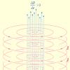
Attention should be paid to some important features of all diffraction paintings. Figure 4.1. It can be seen that in the center of the polar diagram there is a central maximum intensity of scattered radiation. This maximum has a high symmetry close to the symmetry of the limiting group with ¥. In the angular distribution of scattered radiation, the central maximum occupies a certain interval of the polar angles Qî. The semi-width of the central maximum significantly depends on the wavelength of X-rays L and the number of scattering atoms.
It is also very important that the intensity of the central maximum significantly exceeds the intensity of all other points of the two-dimensional angular distribution of multiple x-ray radiation. On the contrary, with an increase in the polar angle, the intensity of scattered radiation in the average falls sharply. This means that the peripheral area of \u200b\u200bthe diffraction pattern (the area of \u200b\u200bpolar angles exceeding a certain value Qm) practically does not affect the magnitude of the coefficient of rotary pseudo-symmetry (4.2).
As a result, the degree of invariance (4.2) the main contribution gives the central maximum. In other words, the high symmetry of the central maximum suppresses the symmetry features of all other characteristic features of the diffraction pattern.
For a detailed study of rotary pseudo-symmetry, the angular distribution of scattered X-ray radiation is advisable to calculate the functionals of the following type:
External integrals in the polar corner have limits that can specify the researcher, which allows to study a rotary pseudo-symmetry at various intervals of the polar corner. In other words, the types of type (4.3) give quantitative estimates of the rotary pseudo-symmetry of the diffraction pattern inside the ring given by the pair of polar angles Q1 and Q2. (See Fig. 4.1).
Naturally split the range of polar angles into subbands of a certain width DQ \u003d Q2 -Q1 and calculate the coefficients of pseudo-symmetry for all such subbands.
Fig.4.1. Ring on the polar diagram of the diffraction pattern, which limits the range of polar corners.
It was indicated above that with computer modeling of the angular distribution of the intensity of scattered X-rays, the function I (Q, F) seems to be a two-dimensional set of numeric values \u200b\u200bI (Ql, jm) for finite discrete kits of the angles Ql \u003d LDQ, L \u003d 1, ... NQ; FM \u003d MDF, M \u003d 1, ... NF. Therefore, when calculating the coefficients of the pseudo-symmetry HA, according to the results of calculating the angular distribution of the intensity of scattered X-rays, double integrals in the expression (4.2) are transformed into double sums
If we are interested in averaged rotary pseudo-symmetry of the entire diffraction pattern, the degree of invariance of the following formula:
If we want to explore a swivel pseudo-symmetry in various subbands of the polar angle (see Fig. 4.1), then it is necessary to calculate the amount of sums for the corresponding intervals of type (4.3). Then the coefficients of pseudo-symmetry are as follows:
where the indices L1 and L2 correspond to the values \u200b\u200bof polar angles Q1 and Q2
q1 \u003d L1 DQ, Q2 \u003d L2 DQ. (4.6)
Specifying certain values \u200b\u200bof the angle of rotation A can be calculated by the coefficients of the pseudo-symmetry HA diffraction patterns for the turns of various orders. If we are interested in the rotary pseudo-symmetry of the N-order, the angle of A is expressed by the ratio.
an \u003d 2p / n. (4.7)
3.1.2. Computer simulation of X-ray scattering on molecules and fragments of crystal structures
In this paper, it was calculated by the characteristics of X-ray radiation, scattered by a finite set of atoms under the diffraction conditions of the Fraunhofer. The primary X-ray radiation seemed flat monochromatic wave with a specific wave vector k0 and wavelength l.
The angular distribution of the intensity of X-rays scattered on a finite set of atoms is represented by the function I (Q, F), depending on the two angles - polar q and azimuthal F. The angles Q and F determine the direction to the detector of scattered X-rays, which in the diffraction diffraction conditions coincides With a wave vector K scattered x-ray wave.
The polar angle q is counted from the direction of the wave vector of the primary X-ray wave. The azimuthal angle f is lowered in the plane perpendicular to the vector K0. Azimuth F is an angle between the projection of the wave vector K of a scattered wave on this plane and an arbitrarily selected azimuth axis.
A set of values \u200b\u200bof the function I (Q, F) for all sorts of values \u200b\u200bof the arguments Q and F is often referred to as the diffraction pattern.
Our task addresses the scattering of X-rays in the "front" hemisphere. Consequently, the polar angle Q belongs to the range ,. Azimuthal angle f accepts values \u200b\u200bin the interval)